
Correlation coefficient and correlation test in R

Introduction
Correlations between variables play an important role in a descriptive analysis. A correlation measures the relationship between two variables, that is, how they are linked to each other. In this sense, a correlation allows to know which variables evolve in the same direction, which ones evolve in the opposite direction, and which ones are independent.
In this article, I show how to compute correlation coefficients, how to perform correlation tests and how to visualize relationships between variables in R.
Correlation is usually computed on two quantitative variables, but it can also be computed on two qualitative ordinal variables.1 See the Chi-square test of independence if you need to study the relationship between two qualitative nominal variables.
If you need to quantify the relationship between two variables, I refer you to the article about linear regression.
Data
In this article, we use the mtcars dataset (loaded by default in R):
# display first 5 observations
head(mtcars, 5)
## mpg cyl disp hp drat wt qsec vs am gear carb
## Mazda RX4 21.0 6 160 110 3.90 2.620 16.46 0 1 4 4
## Mazda RX4 Wag 21.0 6 160 110 3.90 2.875 17.02 0 1 4 4
## Datsun 710 22.8 4 108 93 3.85 2.320 18.61 1 1 4 1
## Hornet 4 Drive 21.4 6 258 110 3.08 3.215 19.44 1 0 3 1
## Hornet Sportabout 18.7 8 360 175 3.15 3.440 17.02 0 0 3 2The variables vs and am are categorical variables, so they are removed for this article:
# remove vs and am variables
library(tidyverse)
dat <- mtcars %>%
  select(-vs, -am)

# display 5 first obs. of new dataset
head(dat, 5)
## mpg cyl disp hp drat wt qsec gear carb
## Mazda RX4 21.0 6 160 110 3.90 2.620 16.46 4 4
## Mazda RX4 Wag 21.0 6 160 110 3.90 2.875 17.02 4 4
## Datsun 710 22.8 4 108 93 3.85 2.320 18.61 4 1
## Hornet 4 Drive 21.4 6 258 110 3.08 3.215 19.44 3 1
## Hornet Sportabout 18.7 8 360 175 3.15 3.440 17.02 3 2Correlation coefficient
Between two variables
The correlation between 2 variables is found with the cor() function.
Suppose we want to compute the correlation between horsepower (hp) and miles per gallon (mpg):
# Pearson correlation between 2 variables
cor(dat$hp, dat$mpg)
## [1] -0.7761684Note that the correlation between variables X and Y is equal to the correlation between variables Y and X so the order of the variables in the cor() function does not matter.
The Pearson correlation is computed by default with the cor() function. If you want to compute the Spearman correlation, add the argument method = "spearman" to the cor() function:
# Spearman correlation between 2 variables
cor(dat$hp, dat$mpg,
  method = "spearman"
)
## [1] -0.8946646The most common correlation methods (Run ?cor for more information about the different methods available in the cor() function) are:
- Pearson correlation is often used for quantitative continuous variables that have a linear relationship
- Spearman correlation (which is actually similar to Pearson but based on the ranked values for each variable rather than on the raw data) is often used to evaluate relationships involving at least one qualitative ordinal variable or two quantitative variables if the link is partially linear
- Kendall’s tau-b which is computed from the number of concordant and discordant pairs is often used for qualitative ordinal variables
Note that there exists the point-biserial correlation (which can be used to measure the association between a continuous variable and a nominal variable of two levels), but this correlation is not covered here.
Correlation matrix: correlations for all variables
Suppose now that we want to compute correlations for several pairs of variables. We can easily do so for all possible pairs of variables in the dataset, again with the cor() function:
# correlation for all variables
round(cor(dat),
  digits = 2 # rounded to 2 decimals
)
## mpg cyl disp hp drat wt qsec gear carb
## mpg 1.00 -0.85 -0.85 -0.78 0.68 -0.87 0.42 0.48 -0.55
## cyl -0.85 1.00 0.90 0.83 -0.70 0.78 -0.59 -0.49 0.53
## disp -0.85 0.90 1.00 0.79 -0.71 0.89 -0.43 -0.56 0.39
## hp -0.78 0.83 0.79 1.00 -0.45 0.66 -0.71 -0.13 0.75
## drat 0.68 -0.70 -0.71 -0.45 1.00 -0.71 0.09 0.70 -0.09
## wt -0.87 0.78 0.89 0.66 -0.71 1.00 -0.17 -0.58 0.43
## qsec 0.42 -0.59 -0.43 -0.71 0.09 -0.17 1.00 -0.21 -0.66
## gear 0.48 -0.49 -0.56 -0.13 0.70 -0.58 -0.21 1.00 0.27
## carb -0.55 0.53 0.39 0.75 -0.09 0.43 -0.66 0.27 1.00This correlation matrix gives an overview of the correlations for all combinations of two variables.
Interpretation of a correlation coefficient
First of all, correlation ranges from -1 to 1. It gives us an indication on two things:
- The direction of the relationship between the 2 variables
- The strength of the relationship between the 2 variables
Regarding the direction of the relationship: On the one hand, a negative correlation implies that the two variables under consideration vary in opposite directions, that is, if a variable increases the other decreases and vice versa. On the other hand, a positive correlation implies that the two variables under consideration vary in the same direction, i.e., if a variable increases the other one increases and if one decreases the other one decreases as well.
Regarding the strength of the relationship: The more extreme the correlation coefficient (the closer to -1 or 1), the stronger the relationship. This also means that a correlation close to 0 indicates that the two variables are independent, that is, as one variable increases, there is no tendency in the other variable to either decrease or increase.
As an illustration, the Pearson correlation between horsepower (hp) and miles per gallon (mpg) found above is -0.78, meaning that the 2 variables vary in opposite direction. This makes sense, cars with more horsepower tend to consume more fuel (and thus have a lower mileage per gallon). On the contrary, from the correlation matrix we see that the correlation between miles per gallon (mpg) and the time to drive 1/4 of a mile (qsec) is 0.42, meaning that fast cars (low qsec) tend to have a worse mileage per gallon (low mpg). This again makes sense as fast cars tend to consume more fuel.
Note that it is a good practice to visualize the type of the relationship between the two variables before interpreting the correlation coefficients. The reason is that the correlation coefficient could be biased due to an outlier or due to the type of link between the two variables.
For instance, see the two Pearson correlation coefficients (denoted by R in the following plots) when the outlier is excluded and included:
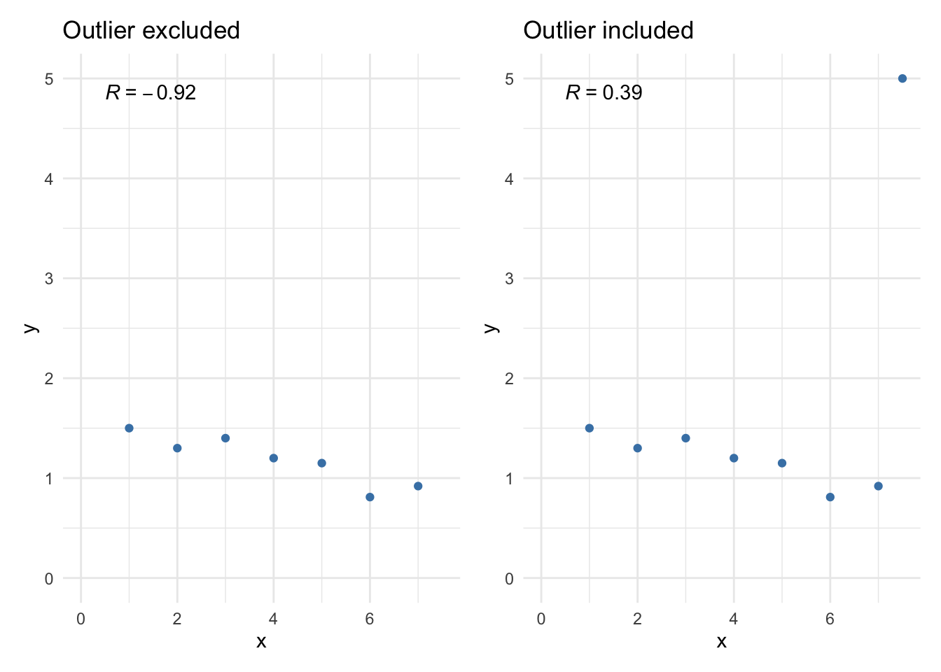
The Pearson correlation coefficient changes drastically due to a single point, and thus the interpretation. It goes from a negative correlation coefficient, indicating a negative relationship between the 2 variables, to a positive coefficient, indicating a positive relationship. We would have missed this insight if we had not visualized the data in a scatterplot (see how to draw a scatterplot in this section).
A correlation coefficient may also miss a non-linear link between two variables:
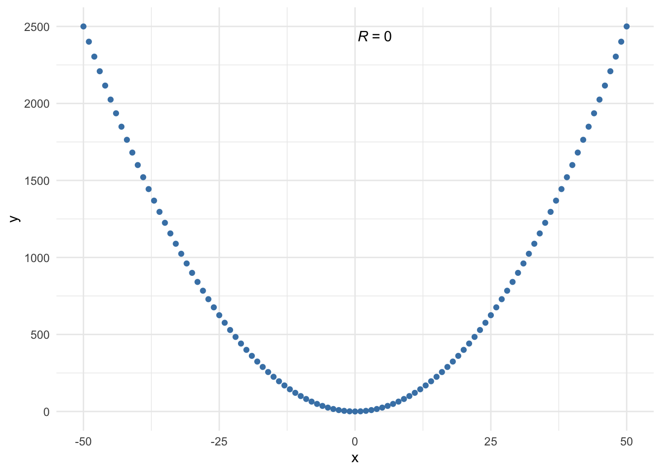
The Pearson correlation coefficient is equal to 0, indicating no relationship between the two variables, because it measures the linear relationship and it is clear from the plot that the link is non-linear.
So to recap, it is a good practice to visualize the data via a scatterplot before interpreting a correlation coefficient (it does not tell the whole story) and see how the correlation coefficient changes when using the parametric (Pearson) or nonparametric version (Spearman or Kendall’s tau-b).
Visualizations
The correlation matrix presented above is not easily interpretable, especially when the dataset is composed of many variables. In the following sections, we present some alternatives to the correlation matrix for better readability.
A scatterplot for 2 variables
A good way to visualize a correlation between 2 variables is to draw a scatterplot of the two variables of interest. Suppose we want to examine the relationship between horsepower (hp) and miles per gallon (mpg):
# scatterplot
library(ggplot2)

ggplot(dat) +
  aes(x = hp, y = mpg) +
  geom_point(colour = "#0c4c8a") +
  theme_minimal()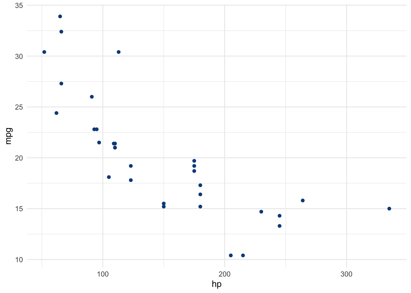
If you are unfamiliar with the {ggplot2} package, you can draw the scatterplot using the plot() function from R base graphics:
plot(dat$hp, dat$mpg)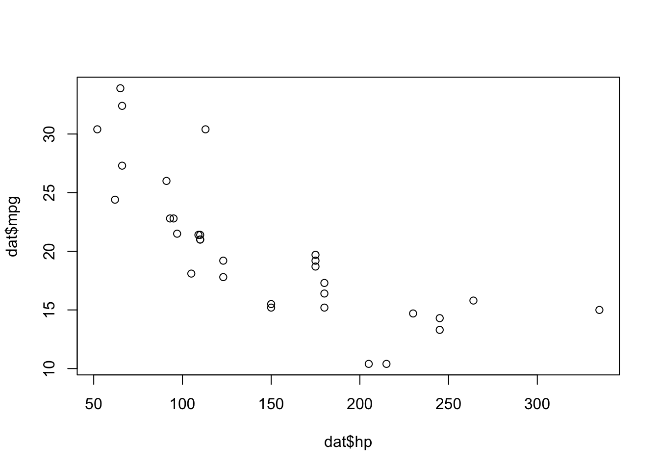
or use the esquisse addin to easily draw plots using the {ggplot2} package.
Scatterplots for several pairs of variables
Suppose that instead of visualizing the relationship between only 2 variables, we want to visualize the relationship for several pairs of variables. This is possible thanks to the pair() function.
For this illustration, we focus only on miles per gallon (mpg), horsepower (hp) and weight (wt):
# multiple scatterplots
pairs(dat[, c("mpg", "hp", "wt")])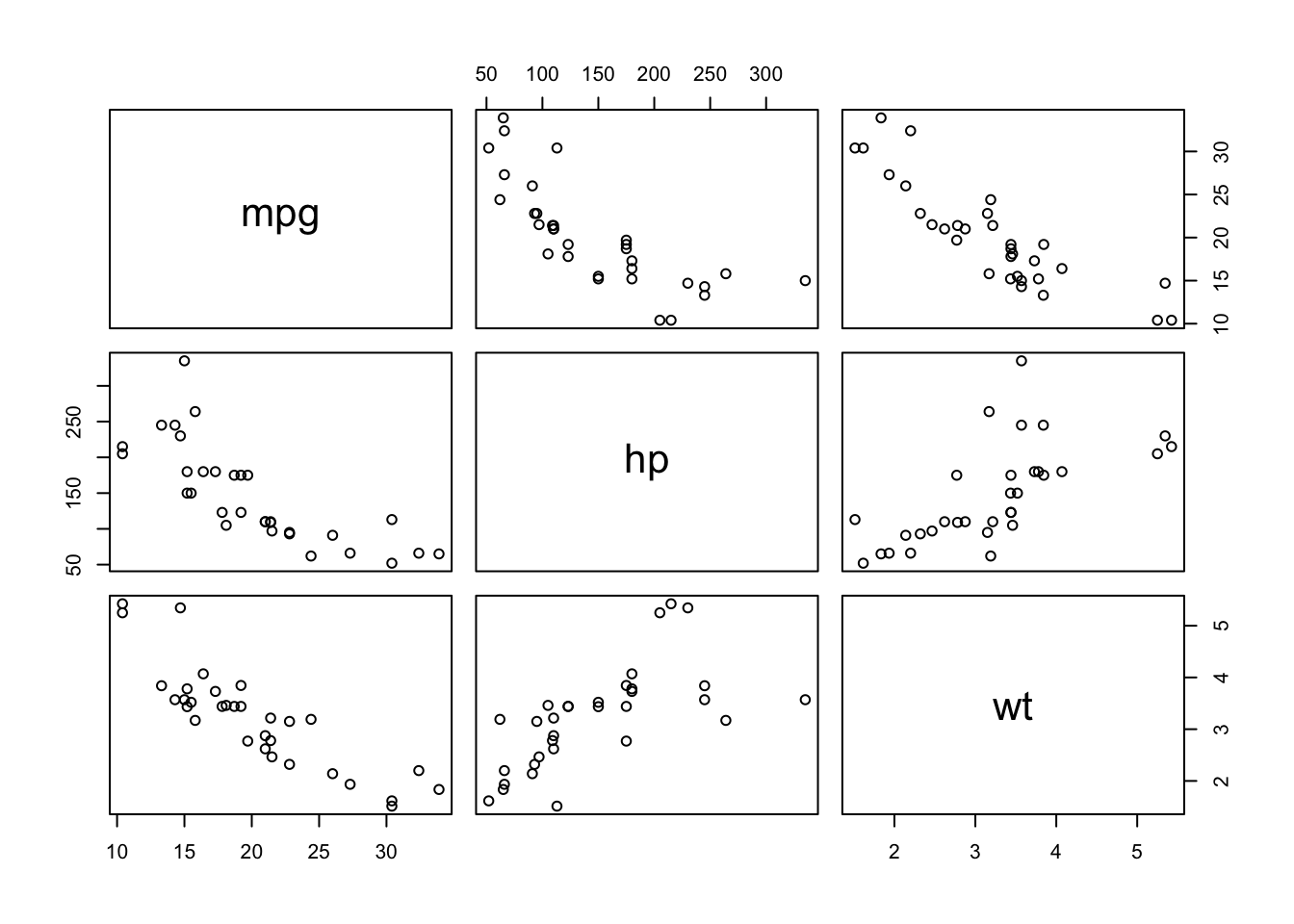
The figure indicates that weight (wt) and horsepower (hp) are positively correlated, whereas miles per gallon (mpg) seems to be negatively correlated with horsepower (hp) and weight (wt).
Another simple correlation matrix
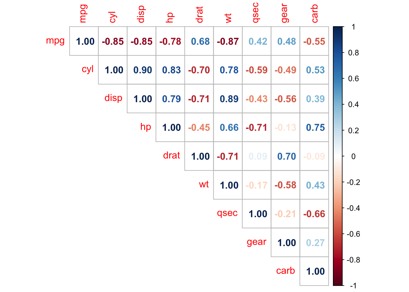
This version of the correlation matrix presents the correlation coefficients in a slightly more readable way, i.e., by coloring the coefficients based on their sign. Applied to our dataset, we have:
# improved correlation matrix
library(corrplot)

corrplot(cor(dat),
  method = "number",
  type = "upper" # show only upper side
)
Correlation test
For 2 variables
Unlike a correlation matrix which indicates the correlation coefficients between some pairs of variables in the sample, a correlation test is used to test whether the correlation (denoted \(\rho\)) between 2 variables is significantly different from 0 or not in the population.
Actually, a correlation coefficient different from 0 in the sample does not mean that the correlation is significantly different from 0 in the population. This needs to be tested with a hypothesis test—and known as the correlation test.
The null and alternative hypothesis for the correlation test are as follows:
- \(H_0\): \(\rho = 0\) (meaning that there is no linear relationship between the two variables)
- \(H_1\): \(\rho \ne 0\) (meaning that there is a linear relationship between the two variables)
Via this correlation test, what we are actually testing is whether:
- the sample contains sufficient evidence to reject the null hypothesis and conclude that the correlation coefficient does not equal 0, so the relationship exists in the population.
- or on the contrary, the sample does not contain enough evidence that the correlation coefficient does not equal 0, so in this case we do not reject the null hypothesis of no relationship between the variables in the population.
Note that there are 2 assumptions for this test to be valid:
- Independence of the data
- For small sample sizes (usually \(n < 30\)), the two variables should follow a normal distribution
Suppose that we want to test whether the rear axle ratio (drat) is correlated with the time to drive a quarter of a mile (qsec):
# Pearson correlation test
test <- cor.test(dat$drat, dat$qsec)
test
##
## Pearson's product-moment correlation
##
## data: dat$drat and dat$qsec
## t = 0.50164, df = 30, p-value = 0.6196
## alternative hypothesis: true correlation is not equal to 0
## 95 percent confidence interval:
## -0.265947 0.426340
## sample estimates:
## cor
## 0.09120476The p-value of the correlation test between these 2 variables is 0.62. At the 5% significance level, we do not reject the null hypothesis of no correlation. We therefore conclude that we do not reject the hypothesis that there is no linear relationship between the 2 variables.2
This test proves that even if the correlation coefficient is different from 0 (the correlation is 0.09 in the sample), it is actually not significantly different from 0 in the population.
Note that the p-value of a correlation test is based on the correlation coefficient and the sample size. The larger the sample size and the more extreme the correlation (closer to -1 or 1), the more likely the null hypothesis of no correlation will be rejected.
With a small sample size, it is thus possible to obtain a relatively large correlation in the sample (based on the correlation coefficient), but still find a correlation not significantly different from 0 in the population (based on the correlation test). For this reason, it is recommended to always perform a correlation test before interpreting a correlation coefficient to avoid flawed conclusions.
For several pairs of variables
Similar to the correlation matrix used to compute correlation for several pairs of variables, the rcorr() function (from the {Hmisc} package) allows to compute p-values of the correlation test for several pairs of variables at once. Applied to our dataset, we have:
# correlation tests for whole dataset
library(Hmisc)
res <- rcorr(as.matrix(dat)) # rcorr() accepts matrices only

# display p-values (rounded to 3 decimals)
round(res$P, 3)
## mpg cyl disp hp drat wt qsec gear carb
## mpg NA 0.000 0.000 0.000 0.000 0.000 0.017 0.005 0.001
## cyl 0.000 NA 0.000 0.000 0.000 0.000 0.000 0.004 0.002
## disp 0.000 0.000 NA 0.000 0.000 0.000 0.013 0.001 0.025
## hp 0.000 0.000 0.000 NA 0.010 0.000 0.000 0.493 0.000
## drat 0.000 0.000 0.000 0.010 NA 0.000 0.620 0.000 0.621
## wt 0.000 0.000 0.000 0.000 0.000 NA 0.339 0.000 0.015
## qsec 0.017 0.000 0.013 0.000 0.620 0.339 NA 0.243 0.000
## gear 0.005 0.004 0.001 0.493 0.000 0.000 0.243 NA 0.129
## carb 0.001 0.002 0.025 0.000 0.621 0.015 0.000 0.129 NAOnly correlations with p-values smaller than the significance level (usually \(\alpha = 0.05\)) should be interpreted.
Combination of correlation coefficients and correlation tests
Now that we covered the concepts of correlation coefficients and correlation tests, let see if we can combine the two concepts.
If you need to do this for a few pairs of variables, I recommend using the ggscatterstats() function from the {ggstatsplot} package. Let’s see it in practice with one pair of variables—wt and mpg:
## plot with statistical results
library(ggstatsplot)

ggscatterstats(
  data = dat,
  x = wt,
  y = mpg,
  bf.message = FALSE,
  marginal = FALSE # remove histograms
)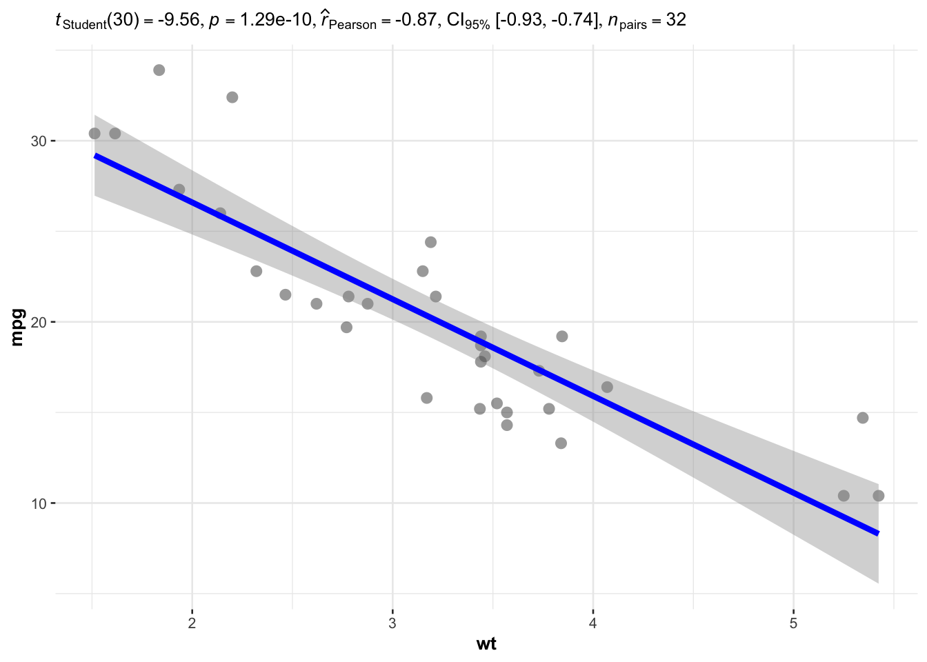
Based on the result of the test, we conclude that there is a negative correlation between the weight and the number of miles per gallon (\(r = - 0.87\), \(p\)-value < 0.001).
If you need to do it for many pairs of variables, I recommend using the the correlation function from the easystats {correlation} package.
This function allows to combine correlation coefficients and correlation tests for several pairs of variables, all in a single table (thanks to krzysiektr for pointing it out to me):
library(correlation)

correlation::correlation(dat,
  include_factors = TRUE, method = "auto"
)
## # Correlation Matrix (auto-method)
##
## Parameter1 | Parameter2 | r | 95% CI | t(30) | p
## --------------------------------------------------------------------
## mpg | cyl | -0.85 | [-0.93, -0.72] | -8.92 | < .001***
## mpg | disp | -0.85 | [-0.92, -0.71] | -8.75 | < .001***
## mpg | hp | -0.78 | [-0.89, -0.59] | -6.74 | < .001***
## mpg | drat | 0.68 | [ 0.44, 0.83] | 5.10 | < .001***
## mpg | wt | -0.87 | [-0.93, -0.74] | -9.56 | < .001***
## mpg | qsec | 0.42 | [ 0.08, 0.67] | 2.53 | 0.137
## mpg | gear | 0.48 | [ 0.16, 0.71] | 3.00 | 0.065
## mpg | carb | -0.55 | [-0.75, -0.25] | -3.62 | 0.016*
## cyl | disp | 0.90 | [ 0.81, 0.95] | 11.45 | < .001***
## cyl | hp | 0.83 | [ 0.68, 0.92] | 8.23 | < .001***
## cyl | drat | -0.70 | [-0.84, -0.46] | -5.37 | < .001***
## cyl | wt | 0.78 | [ 0.60, 0.89] | 6.88 | < .001***
## cyl | qsec | -0.59 | [-0.78, -0.31] | -4.02 | 0.007**
## cyl | gear | -0.49 | [-0.72, -0.17] | -3.10 | 0.054
## cyl | carb | 0.53 | [ 0.22, 0.74] | 3.40 | 0.027*
## disp | hp | 0.79 | [ 0.61, 0.89] | 7.08 | < .001***
## disp | drat | -0.71 | [-0.85, -0.48] | -5.53 | < .001***
## disp | wt | 0.89 | [ 0.78, 0.94] | 10.58 | < .001***
## disp | qsec | -0.43 | [-0.68, -0.10] | -2.64 | 0.131
## disp | gear | -0.56 | [-0.76, -0.26] | -3.66 | 0.015*
## disp | carb | 0.39 | [ 0.05, 0.65] | 2.35 | 0.177
## hp | drat | -0.45 | [-0.69, -0.12] | -2.75 | 0.110
## hp | wt | 0.66 | [ 0.40, 0.82] | 4.80 | < .001***
## hp | qsec | -0.71 | [-0.85, -0.48] | -5.49 | < .001***
## hp | gear | -0.13 | [-0.45, 0.23] | -0.69 | > .999
## hp | carb | 0.75 | [ 0.54, 0.87] | 6.21 | < .001***
## drat | wt | -0.71 | [-0.85, -0.48] | -5.56 | < .001***
## drat | qsec | 0.09 | [-0.27, 0.43] | 0.50 | > .999
## drat | gear | 0.70 | [ 0.46, 0.84] | 5.36 | < .001***
## drat | carb | -0.09 | [-0.43, 0.27] | -0.50 | > .999
## wt | qsec | -0.17 | [-0.49, 0.19] | -0.97 | > .999
## wt | gear | -0.58 | [-0.77, -0.29] | -3.93 | 0.008**
## wt | carb | 0.43 | [ 0.09, 0.68] | 2.59 | 0.132
## qsec | gear | -0.21 | [-0.52, 0.15] | -1.19 | > .999
## qsec | carb | -0.66 | [-0.82, -0.40] | -4.76 | < .001***
## gear | carb | 0.27 | [-0.08, 0.57] | 1.56 | 0.774
##
## p-value adjustment method: Holm (1979)
## Observations: 32As you can see, it gives, among other useful information, the correlation coefficients (column r) and the result of the correlation test (column 95% CI for the confidence interval or p for the \(p\)-value) for all pairs of variables.
Correlograms
The table above is very useful and informative, but let see if it is possible to combine the concepts of correlation coefficients and correlations test in one single visualization. A visualization that would be easy to read and interpret.
Ideally, we would like to have a concise overview of correlations between all possible pairs of variables present in a dataset, with a clear distinction for correlations that are significantly different from 0.
The figure below, known as a correlogram and adapted from the corrplot() function, does precisely this:
# do not edit
corrplot2 <- function(data,
                      method = "pearson",
                      sig.level = 0.05,
                      order = "original",
                      diag = FALSE,
                      type = "upper",
                      tl.srt = 90,
                      number.font = 1,
                      number.cex = 1,
                      mar = c(0, 0, 0, 0)) {
  library(corrplot)
  data_incomplete <- data
  data <- data[complete.cases(data), ]
  mat <- cor(data, method = method)
  cor.mtest <- function(mat, method) {
    mat <- as.matrix(mat)
    n <- ncol(mat)
    p.mat <- matrix(NA, n, n)
    diag(p.mat) <- 0
    for (i in 1:(n - 1)) {
      for (j in (i + 1):n) {
        tmp <- cor.test(mat[, i], mat[, j], method = method)
        p.mat[i, j] <- p.mat[j, i] <- tmp$p.value
      }
    }
    colnames(p.mat) <- rownames(p.mat) <- colnames(mat)
    p.mat
  }
  p.mat <- cor.mtest(data, method = method)
  col <- colorRampPalette(c("#BB4444", "#EE9988", "#FFFFFF", "#77AADD", "#4477AA"))
  corrplot(mat,
    method = "color", col = col(200), number.font = number.font,
    mar = mar, number.cex = number.cex,
    type = type, order = order,
    addCoef.col = "black", # add correlation coefficient
    tl.col = "black", tl.srt = tl.srt, # rotation of text labels
    # combine with significance level
    p.mat = p.mat, sig.level = sig.level, insig = "blank",
    # hide correlation coefficients on the diagonal
    diag = diag
  )
}

# edit from here
corrplot2(
  data = dat,
  method = "pearson",
  sig.level = 0.05,
  order = "original",
  diag = FALSE,
  type = "upper",
  tl.srt = 75
)
The correlogram shows correlation coefficients for all pairs of variables (with more intense colors for more extreme correlations), and correlations not significantly different from 0 are represented by a white box.
To learn more about this plot and the code used, I invite you to read the article entitled “Correlogram in R: how to highlight the most correlated variables in a dataset”.
For those of you who are still not completely satisfied, I recently found two alternatives—one with the ggpairs() function from the {GGally} package and one with the ggcormat() function from the {ggstatsplot} package.
The two functions are illustrated with the variables mpg, hp and wt:
library(GGally)

ggpairs(dat[, c("mpg", "hp", "wt")])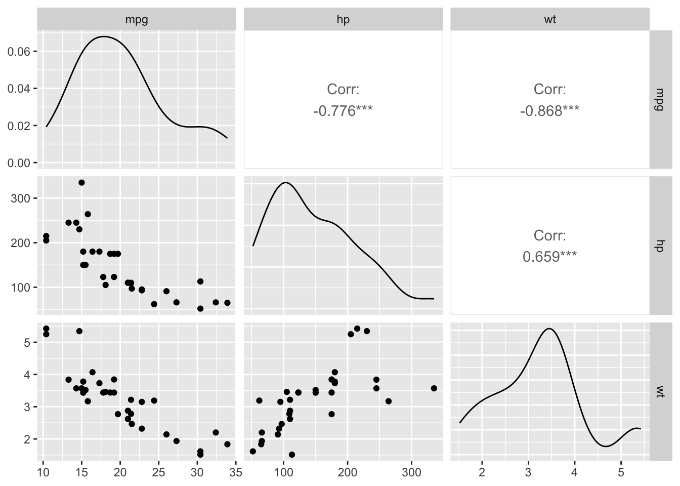
The plot above combines correlation coefficients, correlation tests (via the asterisks next to the coefficients3) and scatterplots for all possible pairs of variables present in a dataset.
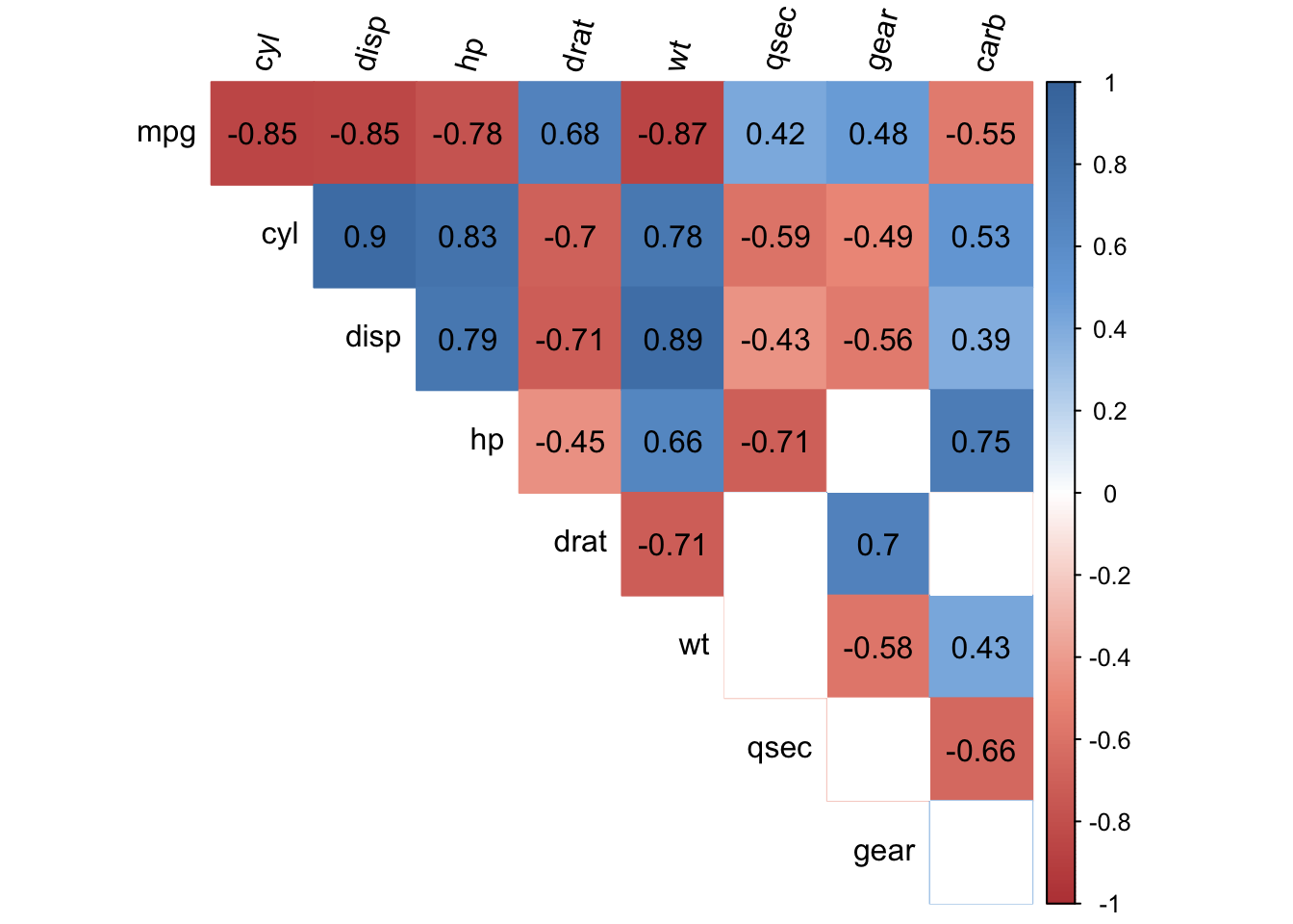
library(ggstatsplot)

ggcorrmat(
  data = dat[, c("mpg", "hp", "wt")],
  type = "parametric", # parametric for Pearson, nonparametric for Spearman's correlation
  colors = c("darkred", "white", "steelblue") # change default colors
)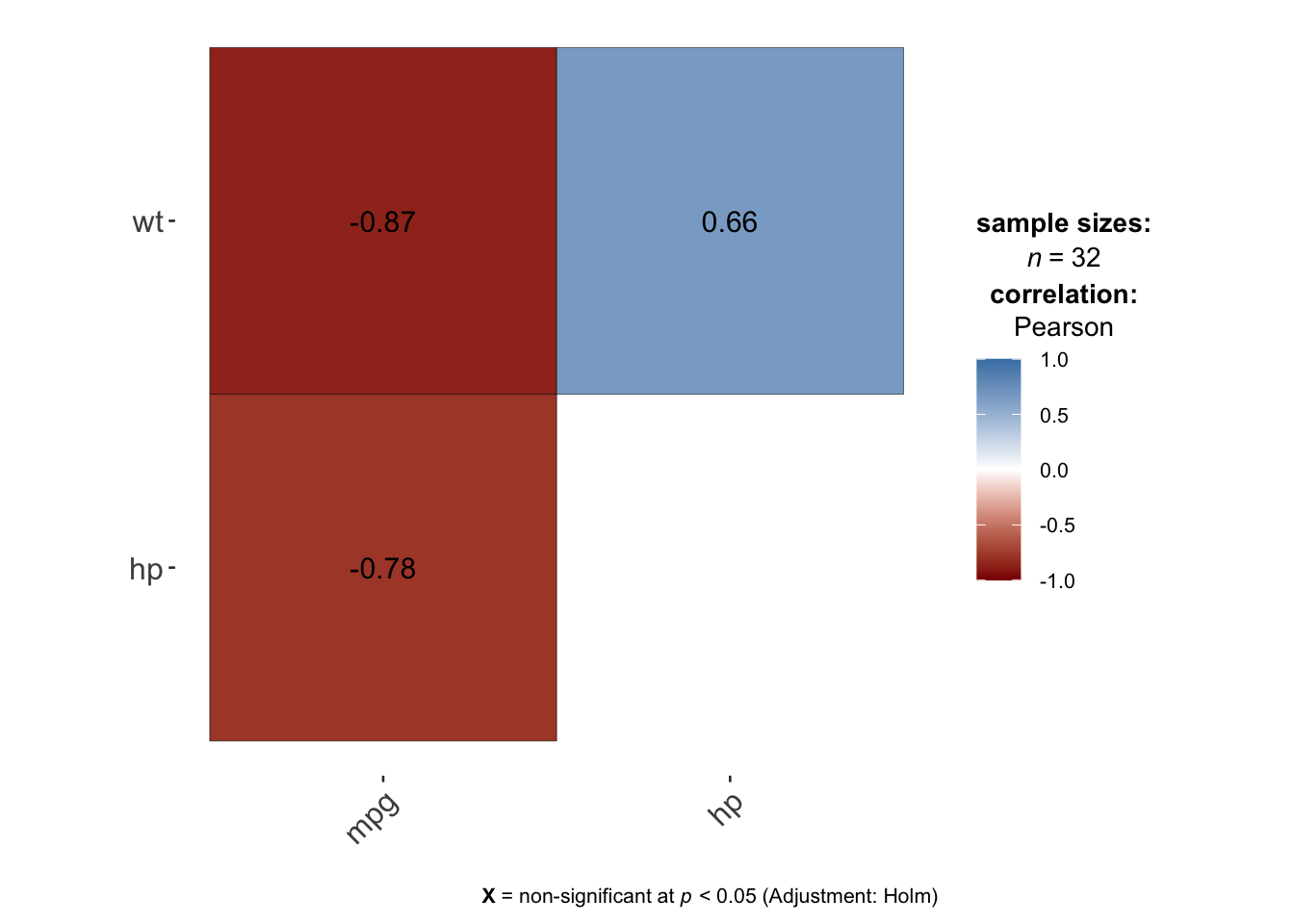
The plot above also shows the correlation coefficients and if any, the non-significant correlations (by default at the 5% significance level with the Holm adjustment method) are shown by a big cross on the correlation coefficients.
The advantage of these two alternatives compared to the first one is that it is directly available within a package, so you do not need to run the code of the function first in order to draw the correlogram.
Correlation does not imply causation
I am pretty sure you have already heard the statement “Correlation does not imply causation” in statistics. An article about correlation would not be complete without discussing about causation.
A non-zero correlation between two variables does not necessarily mean that there is a cause and effect relationship between these two variables!
Indeed, a significant correlation between two variables means that changes in one variable are associated (positively or negatively) with changes in the other variable. Nonetheless, a significant correlation does not indicate that variations in one variable cause the variations in the other variable.
A non-zero correlation between X and Y can appear in several cases:
- X causes Y
- Y causes X
- a third variable causes X and Y
- a combination of these three reasons
Sometimes it is quite clear that there is a causal relationship between two variables. Take for example the correlation between the price of a consumer product such as milk and its consumption. It is quite obvious that there is a causal link between the two: if the price of milk increases, it is expected that its consumption will decrease.
However, this causal link is not always present even if the correlation is significant. Maurage et al. (2013) showed that, although there is a positive and significant correlation between chocolate consumption and the number of Nobel laureates, this correlation comes from the fact that a third variable, Gross Domestic Product (GDP), causes chocolate consumption and the number of Nobel laureates. They found that countries with higher GDP tend to have a higher level of chocolate consumption and scientific research (leading to more Nobel laureates).
This example shows that one must be very cautious when interpreting correlations and avoid over-interpreting a correlation as a causal relationship.
Conclusion
Thanks for reading.
I hope this article helped you to compute correlation coefficients and perform correlation tests in R. If you would like to learn how to compute the coefficients by hand, see this step-by-step tutorial.
As always, if you have a question or a suggestion related to the topic covered in this article, please add it as a comment so other readers can benefit from the discussion.
(Note that this article is available for download on my Gumroad page.)
References
It is true that there is the point-biserial correlation which can be used with a nominal variable (consisting of two factors). Nonetheless, this type of correlation is much less known and usually not covered in introductory statistics classes; with one continuous and one nominal variable, it is much more frequent to learn about the Student’s t-test (for a nominal variable with 2 groups) or ANOVA (for a nominal variable with 3 or more groups). More information about choosing the most appropriate measure of association depending on the type of variable can be found in this article.↩︎
It is important to remember that we tested for a linear relationship between the two variables since we used the Pearson’s correlation. It may be the case that there is a relationship between the two variables in the population, but this relation may not be linear.↩︎
One asterisk means that the coefficient is significant at the 5% level, 2 is at the 1% significance level, and 3 is at the 0.1% significance level. This is usually the case in R; the more asterisks, the more it is significant.↩︎
Liked this post?
- Get updates every time a new article is published (no spam and unsubscribe anytime)
- Support the blog
- Share on:


