
Data manipulation in R
- Introduction
- Vectors
- Factors
- Lists
- Data frames
- Missing values
- Scale
- Dates and times
- Exporting and saving
- Looking for help
- Conclusion

Note that this article is inspired from a workshop entitled “Introduction to data analysis with R”, given by UCLouvain’s Statistical Methodology and Computing Service. See all their workshops on their website.
Introduction
Not all data frames are as clean and tidy as you would expect. Therefore, after importing your data frame into RStudio, most of the time you will need to prepare it before performing any statistical analyses. Data manipulation can even sometimes take longer than the actual analyses when the quality of the data is poor.
Data manipulation include a broad range of tools and techniques. We present here in details the manipulations that you will most likely need for your projects in R. Do not hesitate to let me know (as a comment at the end of this article for example) if you find other data manipulations essential so that I can add them.
In this article we show the main functions to manipulate data in R. We first illustrate these functions on vectors, factors and lists. We then illustrate the main functions to manipulate data frames and dates/times in R.
For those who are interested in going further, see also an introduction to data manipulation in R with the {dplyr} package.
Vectors
Concatenation
We can concatenate (i.e., combine) numbers or strings with c():
c(2, 4, -1)## [1] 2 4 -1c(1, 5 / 6, 2^3, -0.05)## [1] 1.0000000 0.8333333 8.0000000 -0.0500000Note that by default R displays 7 decimals. You can modify it with options(digits = 2) (two decimals).
It is also possible to create a sequence of consecutive integers:
1:10## [1] 1 2 3 4 5 6 7 8 9 10# is the same than
c(1, 2, 3, 4, 5, 6, 7, 8, 9, 10)## [1] 1 2 3 4 5 6 7 8 9 10# or
c(1:10)## [1] 1 2 3 4 5 6 7 8 9 10seq() and rep()
seq() allows to make a vector defined by a sequence. You can either choose the increment:
seq(from = 2, to = 5, by = 0.5)## [1] 2.0 2.5 3.0 3.5 4.0 4.5 5.0or its length:
seq(from = 2, to = 5, length.out = 7)## [1] 2.0 2.5 3.0 3.5 4.0 4.5 5.0On the other hand, rep() creates a vector which is the repetition of numbers or strings:
rep(1, times = 3)## [1] 1 1 1rep(c("A", "B", "C"), times = c(3, 1, 2))## [1] "A" "A" "A" "B" "C" "C"You can also create a vector which is the repetition of numbers and strings:
rep(c("A", 2, "C"), times = c(3, 1, 2))## [1] "A" "A" "A" "2" "C" "C"but in that case, the number 2 will be considered as a string too (and not as a numeric) since there is at least one string in the vector.
Assignment
There are three ways to assign an object in R:
<-=assign()
# 1st method
x <- c(2.1, 5, -4, 1, 5)
x
## [1] 2.1 5.0 -4.0 1.0 5.0# 2nd method
x2 = c(2.1, 5, -4, 1, 5)
x2## [1] 2.1 5.0 -4.0 1.0 5.0# 3rd method (much less common)
assign("x3", c(2.1, 5, -4, 1, 5))
x3## [1] 2.1 5.0 -4.0 1.0 5.0You can also assign a vector to another vector, for example:
y <- c(x, 10, 1 / 4)
y
## [1] 2.10 5.00 -4.00 1.00 5.00 10.00 0.25Elements of a vector
We can select one or several elements of a vector by specifying its position between square brackets:
# select one element
x[3]
## [1] -4# select more than one element with c()
x[c(1, 3, 4)]## [1] 2.1 -4.0 1.0Note that in R the numbering of the indices starts at 1 (and no 0 like other programming languages) so x[1] gives the first element of the vector x.
We can also use booleans (i.e., TRUE or FALSE) to select some elements of a vector. This method selects only the elements corresponding to TRUE:
x[c(TRUE, FALSE, TRUE, TRUE, FALSE)]## [1] 2.1 -4.0 1.0Or we can give the elements to withdraw:
x[-c(2, 4)]## [1] 2.1 -4.0 5.0Type and length
The main types of a vector are numeric, logical and character. For more details on each type, see the different data types in R.
class() gives the vector type:
x <- c(2.1, 5, -4, 1, 5, 0)
class(x)
## [1] "numeric"y <- c(x, "Hello")
class(y)## [1] "character"As you can see above, the class of a vector will be numeric only if all of its elements are numeric. As soon as one element is a character, the class of the vector will be a character.
z <- c(TRUE, FALSE, FALSE)
class(z)
## [1] "logical"length() gives the length of a vector:
length(x)## [1] 6So to select the last element of a vector (in a dynamic way), we can use a combination of length() and []:
x[length(x)]## [1] 0Finding the vector type
We can find the type of a vector with the family of is.type functions:
is.numeric(x)## [1] TRUEis.logical(x)## [1] FALSEis.character(x)## [1] FALSEOr in a more generic way with the is() function:
is(x)## [1] "numeric" "vector"Modifications of type and length
We can change the type of a vector with the as.numeric(), as.logical() and as.character() functions:
x_character <- as.character(x)
x_character
## [1] "2.1" "5" "-4" "1" "5" "0"is.character(x_character)## [1] TRUEx_logical <- as.logical(x)
x_logical## [1] TRUE TRUE TRUE TRUE TRUE FALSEis.logical(x_logical)## [1] TRUEIt is also possible to change its length:
length(x) <- 4
x
## [1] 2.1 5.0 -4.0 1.0As you can see, the first elements of the vector are conserved while all others are removed. In this case, the first 4 since we specified a length of 4.
Numerical operators
The basic numerical operators such as +, -, *, / and ^ can be applied to vectors:
x <- c(2.1, 5, -4, 1)
y <- c(0, -7, 1, 1 / 4)

x + y
## [1] 2.10 -2.00 -3.00 1.25x * y## [1] 0.00 -35.00 -4.00 0.25x^y## [1] 1.00e+00 1.28e-05 -4.00e+00 1.00e+00It is also possible to compute the minimum, maximum, sum, product, cumulative sum and cumulative product of a vector:
min(x)## [1] -4max(x)## [1] 5sum(x)## [1] 4.1prod(x)## [1] -42cumsum(x)## [1] 2.1 7.1 3.1 4.1cumprod(x)## [1] 2.1 10.5 -42.0 -42.0The following mathematical operations can be applied too:
sqrt()(square root)cos()(cosine)sin()(sine)tan()(tangent)log()(logarithm)log10()(base 10 logarithm)exp()(exponential)abs()(absolute value)
cos(x)## [1] -0.5048461 0.2836622 -0.6536436 0.5403023exp(x)## [1] 8.16616991 148.41315910 0.01831564 2.71828183If you need to round a number, you can use the round(), floor() and ceiling() functions:
round(cos(x), digits = 3) # round to 3 decimals## [1] -0.505 0.284 -0.654 0.540floor(cos(x)) # largest integer not greater than x## [1] -1 0 -1 0ceiling(cos(x)) # smallest integer not less than x## [1] 0 1 0 1Logical operators
The most common logical operators in R are:
- Negation:
! - Comparisons:
<,<=,>=,>,==(equality),!=(difference) - And:
& - Or:
|
x## [1] 2.1 5.0 -4.0 1.0x <= c(1, 6, 3, 4)## [1] FALSE TRUE TRUE TRUEx <= 1## [1] FALSE FALSE TRUE TRUE(x == 1 | x > 4)## [1] FALSE TRUE FALSE TRUE!(x == 1 | x > 4)## [1] TRUE FALSE TRUE FALSEall() and any()
As the names suggest, all() return TRUE if conditions are met for all elements, whereas any() returns TRUE if conditions are met for any of the element of a vector:
x## [1] 2.1 5.0 -4.0 1.0x <= 1## [1] FALSE FALSE TRUE TRUEall(x <= 1)## [1] FALSEany(x <= 1)## [1] TRUEOperations on character strings vector
You can paste two vectors (or more) together:
code <- paste(c("BE", "BE", "FR", "EN", "BE"), 1:5, sep = "/")
code
## [1] "BE/1" "BE/2" "FR/3" "EN/4" "BE/5"The argument sep stands for separator and allows to specify the character(s) or symbol(s) used to separate each character strings.
If you do not want to specify a separator, you can use sep = "" or the paste0() function:
paste(c("BE", "BE", "FR", "EN", "BE"), 1:5, sep = "")## [1] "BE1" "BE2" "FR3" "EN4" "BE5"paste0(c("BE", "BE", "FR", "EN", "BE"), 1:5)## [1] "BE1" "BE2" "FR3" "EN4" "BE5"To find the positions of the elements containing a given string, use the grep() function:
grep("BE", code)## [1] 1 2 5To extract a character string based on the beginning and the end positions, we can use the substr() function:
# extract characters 1 to 3
substr(code,
  start = 1,
  stop = 3
)
## [1] "BE/" "BE/" "FR/" "EN/" "BE/"Replace a character string by another one if it exists in the vector by using the sub() function:
sub(
  pattern = "BE", # find BE
  replacement = "BEL", # replace it with BEL
  code
)
## [1] "BEL/1" "BEL/2" "FR/3" "EN/4" "BEL/5"Split a character string based on a specific symbol with the strsplit() function:
strsplit(c("Rafael Nadal", "Roger Federer", "Novak Djokovic"),
  split = " "
)
## [[1]]
## [1] "Rafael" "Nadal"
##
## [[2]]
## [1] "Roger" "Federer"
##
## [[3]]
## [1] "Novak" "Djokovic"strsplit(code,
split = "/"
)## [[1]]
## [1] "BE" "1"
##
## [[2]]
## [1] "BE" "2"
##
## [[3]]
## [1] "FR" "3"
##
## [[4]]
## [1] "EN" "4"
##
## [[5]]
## [1] "BE" "5"To transform a character vector to uppercase and lowercase:
toupper(c("Rafael Nadal", "Roger Federer", "Novak Djokovic"))## [1] "RAFAEL NADAL" "ROGER FEDERER" "NOVAK DJOKOVIC"tolower(c("Rafael Nadal", "Roger Federer", "Novak Djokovic"))## [1] "rafael nadal" "roger federer" "novak djokovic"Orders and vectors
We can sort the elements of a vector from smallest to largest, or from largest to smallest:
x <- c(2.1, 5, -4, 1, 1)
sort(x) # smallest to largest
## [1] -4.0 1.0 1.0 2.1 5.0sort(x, decreasing = TRUE) # largest to smallest## [1] 5.0 2.1 1.0 1.0 -4.0order() gives the permutation to apply to the vector in order to sort its elements:
order(x)## [1] 3 4 5 1 2As you can see, the third element of the vector is the smallest and the second element is the largest. This is indicated by the 3 at the beginning of the output, and the 2 at the end of the output.
Like sort() the decreasing = TRUE argument can also be added:
order(x, decreasing = TRUE)## [1] 2 1 4 5 3In this case, the 2 in the output indicates that the second element of the vector is the largest, while the 3 indicates that the third element is the smallest.
rank() gives the ranks of the elements:
rank(x)## [1] 4.0 5.0 1.0 2.5 2.5The two last elements of the vector have a rank of 2.5 because they are equal and they come after the first but before the fourth rank.
We can also reverse the elements (from the last one to the first one):
x## [1] 2.1 5.0 -4.0 1.0 1.0rev(x)## [1] 1.0 1.0 -4.0 5.0 2.1Factors
Factors in R are vectors with a list of levels, also referred as categories. Factors are useful for qualitative data such as the gender, civil status, eye color, etc.
Creating factors
We create factors with the factor() function (do not forget the c()):
f1 <- factor(c("T1", "T3", "T1", "T2"))
f1
## [1] T1 T3 T1 T2
## Levels: T1 T2 T3We can of course create a factor from an existing vector:
v <- c(1, 1, 0, 1, 0)
v2 <- factor(v,
  levels = c(0, 1),
  labels = c("bad", "good")
)
v2
## [1] good good bad good bad
## Levels: bad goodWe can also specify that the levels are ordered by adding the ordered = TRUE argument:
v2 <- factor(v,
  levels = c(0, 1),
  labels = c("bad", "good"),
  ordered = TRUE
)
v2
## [1] good good bad good bad
## Levels: bad < goodNote that the order of the levels will follow the order that is specified in the labels argument.
Properties
To know the names of the levels:
levels(f1)## [1] "T1" "T2" "T3"For the number of levels:
nlevels(f1)## [1] 3In R, the first level is always the reference level. This reference level can be modified with relevel():
relevel(f1, ref = "T3")## [1] T1 T3 T1 T2
## Levels: T3 T1 T2You see that “T3” is now the first and thus the reference level. Changing the reference level has an impact on the order they are displayed or treated in statistical analyses. Compare, for instance, boxplots with different reference levels.
Handling
To know the frequencies for each level:
table(f1)## f1
## T1 T2 T3
## 2 1 1# or
summary(f1)## T1 T2 T3
## 2 1 1Note that the relative frequencies (i.e., the proportions) can be found with the combination of prop.table() and table() or summary():
prop.table(table(f1))## f1
##   T1   T2   T3
## 0.50 0.25 0.25# or
prop.table(summary(f1))## T1 T2 T3
## 0.50 0.25 0.25Remember that a factor is coded in R as a numeric vector even though it looks like a character one. We can transform a factor into its numerical equivalent with the as.numeric() function:
f1## [1] T1 T3 T1 T2
## Levels: T1 T2 T3as.numeric(f1)## [1] 1 3 1 2And a numeric vector can be transformed into a factor with the as.factor() or factor() function:
num <- 1:4
fac <- as.factor(num)
fac
## [1] 1 2 3 4
## Levels: 1 2 3 4fac2 <- factor(num)
fac2## [1] 1 2 3 4
## Levels: 1 2 3 4The advantage of factor() is that it is possible to specify a name for each level:
fac2 <- factor(num,
  labels = c("bad", "neutral", "good", "very good")
)
fac2
## [1] bad neutral good very good
## Levels: bad neutral good very goodLists
A list is a vector whose elements can be of different natures: a vector, a list, a factor, numeric or character, etc.
Creating lists
The function list() allows to create lists:
tahiti <- list(
  plane = c("Airbus", "Boeing"),
  departure = c("Brussels", "Milan", "Paris"),
  duration = c(15, 11, 14)
)
tahiti
## $plane
## [1] "Airbus" "Boeing"
##
## $departure
## [1] "Brussels" "Milan" "Paris"
##
## $duration
## [1] 15 11 14Handling
There are several methods to extract elements from a list:
tahiti$departure## [1] "Brussels" "Milan" "Paris"# or
tahiti$de## [1] "Brussels" "Milan" "Paris"# or
tahiti[[2]]## [1] "Brussels" "Milan" "Paris"# or
tahiti[["departure"]]## [1] "Brussels" "Milan" "Paris"tahiti[[2]][c(1, 2)]## [1] "Brussels" "Milan"To transform a list into a vector:
v <- unlist(tahiti)
v
## plane1 plane2 departure1 departure2 departure3 duration1 duration2
## "Airbus" "Boeing" "Brussels" "Milan" "Paris" "15" "11"
## duration3
## "14"is.vector(v)## [1] TRUEGetting details on an object
attributes() gives the names of the elements (it can be used on every R object):
attributes(tahiti)## $names
## [1] "plane" "departure" "duration"str() gives a short description about the elements (it can also be used on every R object):
str(tahiti)## List of 3
## $ plane : chr [1:2] "Airbus" "Boeing"
## $ departure: chr [1:3] "Brussels" "Milan" "Paris"
## $ duration : num [1:3] 15 11 14Data frames
Every imported file in R is a data frame (at least if you do not use a package to import your data in R). A data frame is a mix of a list and a matrix: it has the shape of a matrix but the columns can have different classes.
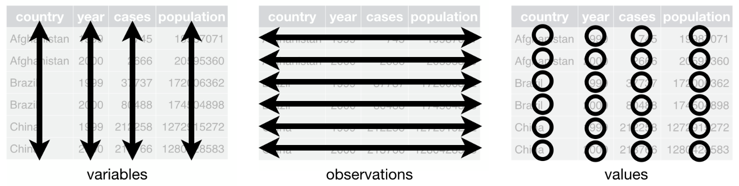
Remember that the gold standard for a data frame is that:
- columns represent variables
- lines correspond to observations and
- each value must have its own cell
In this article, we use the data frame cars to illustrate the main data manipulation techniques. Note that the data frame is installed by default in RStudio (so you do not need to import it) and I use the generic name dat as the name of the data frame throughout the article (see here why I always use a generic name instead of more specific names).
Here is the whole data frame:
dat <- cars # rename the cars data frame with a generic name
dat # display the entire data frame
## speed dist
## 1 4 2
## 2 4 10
## 3 7 4
## 4 7 22
## 5 8 16
## 6 9 10
## 7 10 18
## 8 10 26
## 9 10 34
## 10 11 17
## 11 11 28
## 12 12 14
## 13 12 20
## 14 12 24
## 15 12 28
## 16 13 26
## 17 13 34
## 18 13 34
## 19 13 46
## 20 14 26
## 21 14 36
## 22 14 60
## 23 14 80
## 24 15 20
## 25 15 26
## 26 15 54
## 27 16 32
## 28 16 40
## 29 17 32
## 30 17 40
## 31 17 50
## 32 18 42
## 33 18 56
## 34 18 76
## 35 18 84
## 36 19 36
## 37 19 46
## 38 19 68
## 39 20 32
## 40 20 48
## 41 20 52
## 42 20 56
## 43 20 64
## 44 22 66
## 45 23 54
## 46 24 70
## 47 24 92
## 48 24 93
## 49 24 120
## 50 25 85This data frame has 50 observations with 2 variables (speed and distance).
You can check the number of observations and variables with nrow() and ncol() respectively, or both at the same time with dim():
nrow(dat) # number of rows/observations## [1] 50ncol(dat) # number of columns/variables## [1] 2dim(dat) # dimension: number of rows and number of columns## [1] 50 2Line and column names
Before manipulating a data frame, it is interesting to know the line and column names:
dimnames(dat)## [[1]]
##  [1] "1"  "2"  "3"  "4"  "5"  "6"  "7"  "8"  "9"  "10" "11" "12" "13" "14" "15"
## [16] "16" "17" "18" "19" "20" "21" "22" "23" "24" "25" "26" "27" "28" "29" "30"
## [31] "31" "32" "33" "34" "35" "36" "37" "38" "39" "40" "41" "42" "43" "44" "45"
## [46] "46" "47" "48" "49" "50"
##
## [[2]]
## [1] "speed" "dist"To know only the column names:
names(dat)## [1] "speed" "dist"# or
colnames(dat)## [1] "speed" "dist"And to know only the row names:
rownames(dat)## [1] "1" "2" "3" "4" "5" "6" "7" "8" "9" "10" "11" "12" "13" "14" "15"
## [16] "16" "17" "18" "19" "20" "21" "22" "23" "24" "25" "26" "27" "28" "29" "30"
## [31] "31" "32" "33" "34" "35" "36" "37" "38" "39" "40" "41" "42" "43" "44" "45"
## [46] "46" "47" "48" "49" "50"Subset a data frame
First or last observations
- To keep only the first 10 observations:
head(dat, n = 10)## speed dist
## 1 4 2
## 2 4 10
## 3 7 4
## 4 7 22
## 5 8 16
## 6 9 10
## 7 10 18
## 8 10 26
## 9 10 34
## 10 11 17- To keep only the last 5 observations:
tail(dat, n = 5)## speed dist
## 46 24 70
## 47 24 92
## 48 24 93
## 49 24 120
## 50 25 85Random sample of observations
- To draw a sample of 4 observations without replacement:
library(dplyr)
sample_n(dat, 4, replace = FALSE)
## speed dist
## 1 24 120
## 2 19 46
## 3 4 2
## 4 15 26Based on row or column numbers
If you know what observation(s) or column(s) you want to keep, you can use the row or column number(s) to subset your data frame. We illustrate this with several examples:
- keep all the variables for the \(3^{rd}\) observation:
dat[3, ]- keep the \(2^{nd}\) variable for all observations:
dat[, 2]- You can mix the two above methods to keep only the \(2^{nd}\) variable of the \(3^{rd}\) observation:
dat[3, 2]## [1] 4- keep several observations; for example observations \(1\) to \(5\), the \(10^{th}\) and the \(15^{th}\) observation for all variables:
dat[c(1:5, 10, 15), ] # do not forget c()## speed dist
## 1 4 2
## 2 4 10
## 3 7 4
## 4 7 22
## 5 8 16
## 10 11 17
## 15 12 28- remove observations 5 to 45:
dat[-c(5:45), ]## speed dist
## 1 4 2
## 2 4 10
## 3 7 4
## 4 7 22
## 46 24 70
## 47 24 92
## 48 24 93
## 49 24 120
## 50 25 85- tip: to keep only the last observation, use
nrow()instead of the row number:
dat[nrow(dat), ] # nrow() gives the number of rows## speed dist
## 50 25 85This way, no matter the number of observations, you will always select the last one. This technique of using a piece of code instead of a specific value is to avoid “hard coding”. Hard coding is generally not recommended (unless you want to specify a parameter that you are sure will never change) because if your data frame changes, you will need to manually edit your code.
As you probably figured out by now, you can select observations and/or variables of a dataset by running dataset_name[row_number, column_number]. When the row (column) number is left empty, the entire row (column) is selected.
Note that all examples presented above also work for matrices:
mat <- matrix(c(-1, 2, 0, 3), ncol = 2, nrow = 2)
mat
## [,1] [,2]
## [1,] -1 0
## [2,] 2 3mat[1, 2]## [1] 0Based on variable names
To select one variable of the dataset based on its name rather than on its column number, use dataset_name$variable_name:
dat$speed## [1] 4 4 7 7 8 9 10 10 10 11 11 12 12 12 12 13 13 13 13 14 14 14 14 15 15
## [26] 15 16 16 17 17 17 18 18 18 18 19 19 19 20 20 20 20 20 22 23 24 24 24 24 25Accessing variables inside a data frame with this second method is strongly recommended compared to the first if you intend to modify the structure of your database. Indeed, if a column is added or removed in the data frame, the numbering will change. Therefore, variables are generally referred to by its name rather than by its position (column number). In addition, it is easier to understand and interpret code with the name of the variable written (another reason to call variables with a concise but clear name). There is only one reason why I would still use the column number; if the variables names are expected to change while the structure of the data frame will not change.
To select variables, it is also possible to use the select() command from the powerful dplyr package (for compactness only the first 6 observations are displayed thanks to the head() command):
head(select(dat, speed))## speed
## 1 4
## 2 4
## 3 7
## 4 7
## 5 8
## 6 9This is equivalent than removing the distance variable:
head(select(dat, -dist))## speed
## 1 4
## 2 4
## 3 7
## 4 7
## 5 8
## 6 9Based on one or multiple criterion
Instead of subsetting a data frame based on row/column numbers or variable names, you can also subset it based on one or multiple criterion:
- keep only observations with speed larger than 20. The first argument refers to the name of the data frame, while the second argument refers to the subset criteria:
subset(dat, dat$speed > 20)## speed dist
## 44 22 66
## 45 23 54
## 46 24 70
## 47 24 92
## 48 24 93
## 49 24 120
## 50 25 85- keep only observations with distance smaller than or equal to 50 and speed equal to 10. Note the
==(and not=) for the equal criteria:
subset(dat, dat$dist <= 50 & dat$speed == 10)## speed dist
## 7 10 18
## 8 10 26
## 9 10 34- use
|to keep only observations with distance smaller than 20 or speed equal to 10:
subset(dat, dat$dist < 20 | dat$speed == 10)## speed dist
## 1 4 2
## 2 4 10
## 3 7 4
## 5 8 16
## 6 9 10
## 7 10 18
## 8 10 26
## 9 10 34
## 10 11 17
## 12 12 14- to filter out some observations, use
!=. For instance, to keep observations with speed not equal to 24 and distance not equal to 120 (for compactness only the last 6 observations are displayed thanks to thetail()command):
tail(subset(dat, dat$speed != 24 & dat$dist != 120))## speed dist
## 41 20 52
## 42 20 56
## 43 20 64
## 44 22 66
## 45 23 54
## 50 25 85Note that it is also possible to subset a data frame with split():
split(dat, dat$factor_variable)The above code will split your data frame into several lists, one for each level of the factor variable.
Create a new variable
Often, a data frame can be enhanced by creating new variables based on other variables from the initial data frame, or simply by adding a new variable manually.
In this example, we create two new variables; one being the speed times the distance (which we call speed_dist) and the other being a categorization of the speed (which we call speed_cat). We then display the first 6 observations of this new data frame with the 4 variables:
# create new variable speed_dist
dat$speed_dist <- dat$speed * dat$dist

# create new variable speed_cat
# with ifelse(): if dat$speed > 7, then speed_cat is "high speed", otherwise it is "low_speed"
dat$speed_cat <- factor(ifelse(dat$speed > 7,
  "high speed", "low speed"
))

# display first 6 observations
head(dat) # 6 is the default in head()
## speed dist speed_dist speed_cat
## 1 4 2 8 low speed
## 2 4 10 40 low speed
## 3 7 4 28 low speed
## 4 7 22 154 low speed
## 5 8 16 128 high speed
## 6 9 10 90 high speedNote than in programming, a character string is generally surrounded by quotes (e.g., "character string") and R is not an exception.
Transform a continuous variable into a categorical variable
To transform a continuous variable into a categorical variable (also known as qualitative variable):
dat$speed_quali <- cut(dat$speed,
  breaks = c(0, 12, 15, 19, 26), # cut points
  right = FALSE # closed on the left, open on the right
)

dat[c(1:2, 23:24, 49:50), ] # display some observations
## speed dist speed_dist speed_cat speed_quali
## 1 4 2 8 low speed [0,12)
## 2 4 10 40 low speed [0,12)
## 23 14 80 1120 high speed [12,15)
## 24 15 20 300 high speed [15,19)
## 49 24 120 2880 high speed [19,26)
## 50 25 85 2125 high speed [19,26)This transformation is for example often done on age, when the age (a continuous variable) is transformed into a qualitative variable representing different age groups.
Sum and mean in rows
In survey with Likert scale (used in psychology, among others), it is often the case that we need to compute a score for each respondents based on multiple questions. The score is usually the mean or the sum of all the questions of interest.
This can be done with rowMeans() and rowSums(). For instance, let’s compute the mean and the sum of the variables speed, dist and speed_dist (variables must be numeric of course as a sum and a mean cannot be computed on qualitative variables!) for each row and store them under the variables mean_score and total_score:
dat$mean_score <- rowMeans(dat[, 1:3]) # variables speed, dist and speed_dist correspond to variables 1 to 3
dat$total_score <- rowSums(dat[, 1:3])

head(dat)
## speed dist speed_dist speed_cat speed_quali mean_score total_score
## 1 4 2 8 low speed [0,12) 4.666667 14
## 2 4 10 40 low speed [0,12) 18.000000 54
## 3 7 4 28 low speed [0,12) 13.000000 39
## 4 7 22 154 low speed [0,12) 61.000000 183
## 5 8 16 128 high speed [0,12) 50.666667 152
## 6 9 10 90 high speed [0,12) 36.333333 109Sum and mean in column
It is also possible to compute the mean and sum by column with colMeans() and colSums():
colMeans(dat[, 1:3])## speed dist speed_dist
## 15.40 42.98 769.64colSums(dat[, 1:3])## speed dist speed_dist
## 770 2149 38482This is equivalent than:
mean(dat$speed)## [1] 15.4sum(dat$speed)## [1] 770but it allows to do it for several variables at a time.
Categorical variables and labels management
For categorical variables, it is a good practice to use the factor format and to name the different levels of the variables.
- for this example, let’s create another new variable called
dist_catbased on the distance and then change its format from numeric to factor (while also specifying the labels of the levels):
# create new variable dist_cat
dat$dist_cat <- ifelse(dat$dist < 15,
  1, 2
)

# change from numeric to factor and specify the labels
dat$dist_cat <- factor(dat$dist_cat,
  levels = c(1, 2),
  labels = c("small distance", "big distance") # follow the order of the levels
)

head(dat)
## speed dist speed_dist speed_cat speed_quali mean_score total_score
## 1 4 2 8 low speed [0,12) 4.666667 14
## 2 4 10 40 low speed [0,12) 18.000000 54
## 3 7 4 28 low speed [0,12) 13.000000 39
## 4 7 22 154 low speed [0,12) 61.000000 183
## 5 8 16 128 high speed [0,12) 50.666667 152
## 6 9 10 90 high speed [0,12) 36.333333 109
## dist_cat
## 1 small distance
## 2 small distance
## 3 small distance
## 4 big distance
## 5 big distance
## 6 small distance- to check the format of a variable:
class(dat$dist_cat)## [1] "factor"# or
str(dat$dist_cat)## Factor w/ 2 levels "small distance",..: 1 1 1 2 2 1 2 2 2 2 ...This will be sufficient if you need to format only a limited number of variables. However, if you need to do it for a large amount of categorical variables, it quickly becomes time consuming to write the same code many times. As you can imagine, it possible to format many variables without having to write the entire code for each variable one by one by using the within() command:
dat <- within(dat, {
  speed_cat <- factor(speed_cat, labels = c(
    "high speed",
    "low speed"
  ))
  dist_cat <- factor(dist_cat, labels = c(
    "small distance",
    "big distance"
  ))
})

head(dat)
## speed dist speed_dist speed_cat speed_quali mean_score total_score
## 1 4 2 8 low speed [0,12) 4.666667 14
## 2 4 10 40 low speed [0,12) 18.000000 54
## 3 7 4 28 low speed [0,12) 13.000000 39
## 4 7 22 154 low speed [0,12) 61.000000 183
## 5 8 16 128 high speed [0,12) 50.666667 152
## 6 9 10 90 high speed [0,12) 36.333333 109
## dist_cat
## 1 small distance
## 2 small distance
## 3 small distance
## 4 big distance
## 5 big distance
## 6 small distancestr(dat)## 'data.frame': 50 obs. of 8 variables:
## $ speed : num 4 4 7 7 8 9 10 10 10 11 ...
## $ dist : num 2 10 4 22 16 10 18 26 34 17 ...
## $ speed_dist : num 8 40 28 154 128 90 180 260 340 187 ...
## $ speed_cat : Factor w/ 2 levels "high speed","low speed": 2 2 2 2 1 1 1 1 1 1 ...
## $ speed_quali: Factor w/ 4 levels "[0,12)","[12,15)",..: 1 1 1 1 1 1 1 1 1 1 ...
## $ mean_score : num 4.67 18 13 61 50.67 ...
## $ total_score: num 14 54 39 183 152 109 208 296 384 215 ...
## $ dist_cat : Factor w/ 2 levels "small distance",..: 1 1 1 2 2 1 2 2 2 2 ...Alternatively, if you want to transform several numeric variables into categorical variables without changing the labels, it is best to use the transform() function. We illustrate this function with the mpg data frame from the {ggplot2} package:
library(ggplot2)
mpg <- transform(mpg,
  cyl = factor(cyl),
  drv = factor(drv),
  fl = factor(fl),
  class = factor(class)
)
Recode categorical variables
It is possible to recode labels of a categorical variable if you are not satisfied with the current labels. In this example, we change the labels as follows:
- “small distance” becomes “short distance”
- “big distance” becomes “large distance”
dat$dist_cat <- recode(dat$dist_cat,
  "small distance" = "short distance",
  "big distance" = "large distance"
)

head(dat)
## speed dist speed_dist speed_cat speed_quali mean_score total_score
## 1 4 2 8 low speed [0,12) 4.666667 14
## 2 4 10 40 low speed [0,12) 18.000000 54
## 3 7 4 28 low speed [0,12) 13.000000 39
## 4 7 22 154 low speed [0,12) 61.000000 183
## 5 8 16 128 high speed [0,12) 50.666667 152
## 6 9 10 90 high speed [0,12) 36.333333 109
## dist_cat
## 1 short distance
## 2 short distance
## 3 short distance
## 4 large distance
## 5 large distance
## 6 short distanceChange reference level
For some analyses, you might want to change the order of the levels. For example, if you are analyzing data about a control group and a treatment group, you may want to set the control group as the reference group. By default, levels are ordered by alphabetical order or by its numeric value if it was transformed from numeric to factor.
- to check the current order of the levels (the first level being the reference):
levels(dat$dist_cat)## [1] "short distance" "large distance"In this case, “short distance” being the first level it is the reference level. It is the first level because it was initially set with a value equal to 1 when creating the variable.
- to change the reference level:
dat$dist_cat <- relevel(dat$dist_cat, ref = "large distance")

levels(dat$dist_cat)
## [1] "large distance" "short distance"Large distance is now the first and thus the reference level.
Rename variable names
To rename variable names as follows:
- dist \(\rightarrow\) distance
- speed_dist \(\rightarrow\) speed_distance
- dist_cat \(\rightarrow\) distance_cat
use the rename() command from the dplyr package:
dat <- rename(dat,
  distance = dist,
  speed_distance = speed_dist,
  distance_cat = dist_cat
)

names(dat) # display variable names
## [1] "speed" "distance" "speed_distance" "speed_cat"
## [5] "speed_quali" "mean_score" "total_score" "distance_cat"Create a data frame manually
Although most analyses are performed on an imported data frame, it is also possible to create a data frame directly in R:
# Create the data frame named dat with 2 variables
dat <- data.frame(
  "variable1" = c(6, 12, NA, 3), # presence of 1 missing value (NA)
  "variable2" = c(3, 7, 9, 1)
)

# Print the data frame
dat
## variable1 variable2
## 1 6 3
## 2 12 7
## 3 NA 9
## 4 3 1Merging two data frames
By default, the merge is done on the common variables (variables that have the same name). However, if they do not have the same name, it is still possible to merge the two data frames by specifying their names:
dat1 <- data.frame(
  person = c(1:4),
  treatment = c("T1", "T2")
)

dat1
## person treatment
## 1 1 T1
## 2 2 T2
## 3 3 T1
## 4 4 T2dat2 <- data.frame(
patient = c(1:4),
age = c(56, 23, 32, 19),
gender = c("M", "F", "F", "M")
)
dat2## patient age gender
## 1 1 56 M
## 2 2 23 F
## 3 3 32 F
## 4 4 19 MWe want to merge the two data frames by the subject number, but this number is referred as person in the first data frame and patient in the second data frame, so we need to indicate it:
merge(
  x = dat1, y = dat2,
  by.x = "person", by.y = "patient",
  all = TRUE
)
## person treatment age gender
## 1 1 T1 56 M
## 2 2 T2 23 F
## 3 3 T1 32 F
## 4 4 T2 19 MAdd new observations from another data frame
In order to add new observations from another data frame, the two data frames need to have the same column names (but they can be in a different order):
dat1## person treatment
## 1 1 T1
## 2 2 T2
## 3 3 T1
## 4 4 T2dat3 <- data.frame(
person = 5:8,
treatment = c("T3")
)
dat3## person treatment
## 1 5 T3
## 2 6 T3
## 3 7 T3
## 4 8 T3rbind(dat1, dat3) # r stands for row, so we bind data frames by row## person treatment
## 1 1 T1
## 2 2 T2
## 3 3 T1
## 4 4 T2
## 5 5 T3
## 6 6 T3
## 7 7 T3
## 8 8 T3As you can see, data for persons 5 to 8 have been added at the end of the data frame dat1 (because dat1 comes before dat3 in the rbind() function).
Add new variables from another data frame
It is also possible to add new variables to a data frame with the cbind() function. Unlike rbind(), column names do not have to be the same since they are added next to each other:
dat2## patient age gender
## 1 1 56 M
## 2 2 23 F
## 3 3 32 F
## 4 4 19 Mdat3## person treatment
## 1 5 T3
## 2 6 T3
## 3 7 T3
## 4 8 T3cbind(dat2, dat3) # c stands for column, so we bind data frames by column## patient age gender person treatment
## 1 1 56 M 5 T3
## 2 2 23 F 6 T3
## 3 3 32 F 7 T3
## 4 4 19 M 8 T3If you want to add only a specific variable from another data frame:
dat_cbind <- cbind(dat2, dat3$treatment)

dat_cbind
## patient age gender dat3$treatment
## 1 1 56 M T3
## 2 2 23 F T3
## 3 3 32 F T3
## 4 4 19 M T3names(dat_cbind)[4] <- "treatment"
dat_cbind## patient age gender treatment
## 1 1 56 M T3
## 2 2 23 F T3
## 3 3 32 F T3
## 4 4 19 M T3or more simply with the data.frame() function:
data.frame(dat2,
  treatment = dat3$treatment
)
## patient age gender treatment
## 1 1 56 M T3
## 2 2 23 F T3
## 3 3 32 F T3
## 4 4 19 M T3Missing values
Missing values (represented by NA in RStudio, for “Not Applicable”) are often problematic for many analyses because many computations including a missing value has a missing value for result.
For instance, the mean of a series or variable with at least one NA will give a NA as a result. The data frame dat created in the previous section is used for this example:
dat## variable1 variable2
## 1 6 3
## 2 12 7
## 3 NA 9
## 4 3 1mean(dat$variable1)## [1] NAThe na.omit() function avoids the NA result, doing as if there was no missing value:
mean(na.omit(dat$variable1))## [1] 7Moreover, most basic functions include an argument to deal with missing values:
mean(dat$variable1, na.rm = TRUE)## [1] 7is.na() indicates if an element is a missing value or not:
is.na(dat)## variable1 variable2
## [1,] FALSE FALSE
## [2,] FALSE FALSE
## [3,] TRUE FALSE
## [4,] FALSE FALSENote that “NA” as a string is not considered as a missing value:
y <- c("NA", "2")

is.na(y)
## [1] FALSE FALSETo check whether there is at least one missing value in a vector or data frame:
anyNA(dat$variable2) # check for NA in variable2## [1] FALSEanyNA(dat) # check for NA in the whole data frame## [1] TRUE# or
any(is.na(dat)) # check for NA in the whole data frame## [1] TRUENonetheless, data frames with NAs are still problematic for some types of analysis. Several alternatives exist to remove or impute missing values.
Remove NAs
A simple solution is to remove all observations (i.e., rows) containing at least one missing value. This is done by keeping only observations with complete cases:
dat_complete <- dat[complete.cases(dat), ]
dat_complete
## variable1 variable2
## 1 6 3
## 2 12 7
## 4 3 1Be careful when removing observations with missing values, especially if missing values are not “missing at random”. It is not because it is possible (and easy) to remove them, that you should do it in all cases. This is, however, beyond the scope of the present article.
Impute NAs
Instead of removing observations with at least one NA, it is possible to impute them, that is, replace them by some values such as the median or the mode of the variable. This can be done easily with the command impute() from the package Hmisc:
library(Hmisc)

# impute NA with default method (median/mode)
variable1 <- impute(dat$variable1)

# create data frame with imputed data
dat_imputed <- data.frame(variable1,
  variable2 = dat$variable2
)

dat_imputed
## variable1 variable2
## 1 6 3
## 2 12 7
## 3 6 9
## 4 3 1When the median/mode method is used (the default), character vectors and factors are imputed with the mode. Numeric and integer vectors are imputed with the median. Again, use imputations carefully. Other packages offer more advanced imputation techniques. However, we keep it simple and straightforward for this article as advanced imputations is beyond the scope of introductory data manipulations in R.
Scale
Scaling (also referred as standardizing) a variable is often used before a Principal Component Analysis (PCA)1 when variables of a data frame have different units. Remember that scaling a variable means that it will compute the mean and the standard deviation of that variable. Then each value (so each row) of that variable is “scaled” by subtracting the mean and dividing by the standard deviation of that variable. Formally:
\[z = \frac{x - \bar{x}}{s}\]
where \(\bar{x}\) and \(s\) are the mean and the standard deviation of the variable, respectively.
To scale one or more variables in R use scale():
dat_scaled <- scale(dat_imputed)

head(dat_scaled)
## variable1 variable2
## 1 -0.1986799 -0.5477226
## 2 1.3907590 0.5477226
## 3 -0.1986799 1.0954451
## 4 -0.9933993 -1.0954451Dates and times
Dates
In R the default date format follows the rules of the ISO 8601 international standard which expresses a day as “2001-02-13” (yyyy-mm-dd).2
Date can be defined by a string of characters or a number. For example, October 1st, 2016:
as.Date("01/10/16", format = "%d/%m/%y")## [1] "2016-10-01"as.Date(274, origin = "2016-01-01") # there are 274 days between the origin and October 1st, 2016## [1] "2016-10-01"Times
An example with date and time vectors:
dates <- c("02/27/92", "02/27/99", "01/14/92")
times <- c("23:03:20", "22:29:56", "01:03:30")

x <- paste(dates, times)
x
## [1] "02/27/92 23:03:20" "02/27/99 22:29:56" "01/14/92 01:03:30"strptime(x,
format = "%m/%d/%y %H:%M:%S"
)## [1] "1992-02-27 23:03:20 CET" "1999-02-27 22:29:56 CET"
## [3] "1992-01-14 01:03:30 CET"Find more information on how to express a date and time format with help(strptime).
Extraction from dates
We can extract:
- weekdays
- months
- quarters
- years
y <- strptime(x,
  format = "%m/%d/%y %H:%M:%S"
)

y
## [1] "1992-02-27 23:03:20 CET" "1999-02-27 22:29:56 CET"
## [3] "1992-01-14 01:03:30 CET"weekdays(y, abbreviate = FALSE)## [1] "Thursday" "Saturday" "Tuesday"months(y, abbreviate = FALSE)## [1] "February" "February" "January"quarters(y, abbreviate = FALSE)## [1] "Q1" "Q1" "Q1"format(y, "%Y") # 4-digit year## [1] "1992" "1999" "1992"format(y, "%y") # 2-digit year## [1] "92" "99" "92"Exporting and saving
If a copy-paste is not sufficient, you can save an object in R format with save():
save(dat, file = "dat.Rdata")or using write.table(), write.csv() or write.xlsx():
# in a text format
write.table(dat, "dat.txt", row = FALSE, sep = "\t", quote = FALSE)

# in csv
write.csv(dat, file = "dat.csv", row.names = FALSE, quote = FALSE)

# in excel
# install.packages("openxlsx")
library(openxlsx)
write.xlsx(dat, file = "dat.xlsx")
If you need to send every results into a file instead of the console:
sink("filename")(Don’t forget to stop it with sink().)
Looking for help
You can always find some help about:
- a function:
?functionorhelp(function) - a package:
help(package = packagename) - a concept:
help.search("concept")orapropos("concept")
Otherwise, Google is your best friend!
Conclusion
Thanks for reading.
I hope this article helped you to manipulate your data in RStudio. For those who are interested in going further, see also an introduction to data manipulation in R with the {dplyr} package.
Now that you know how to import a data frame into R and how to manipulate it, the next step would probably be to learn how to perform descriptive statistics in R. If you are looking for more advanced statistical analyses using R, see all articles about R.
As always, if you have a question or a suggestion related to the topic covered in this article, please add it as a comment so other readers can benefit from the discussion.
Principal Component Analysis (PCA) is a useful technique for exploratory data analysis, allowing a better visualization of the variation present in a data frame with a large number of variables. When there are many variables, the data cannot easily be illustrated in their raw format. To counter this, the PCA takes a data frame with many variables and simplifies it by transforming the original variables into a smaller number of “principal components”. The first dimension contains the most variance in the data frame and so on, and the dimensions are uncorrelated. Note that PCA is done on quantitative variables.↩︎
For your information, note that this date format is not the same for every software! Excel, for instance, uses a different format.↩︎
Liked this post?
- Get updates every time a new article is published (no spam and unsubscribe anytime)
- Support the blog
- Share on:


