
How to do a t-test or ANOVA for more than one variable at once in R?

Introduction
As part of my teaching assistant position in a Belgian university, students often ask me for some help in their statistical analyses for their master’s thesis.
A frequent question is how to compare groups of patients in terms of several quantitative continuous variables. Most of us know that:
- To compare two groups, a Student’s t-test should be used1
- To compare three groups or more, an ANOVA should be performed
These two tests are quite basic and have been extensively documented online and in statistical textbooks so the difficulty is not in how to perform these tests.
In the past, I used to do the analyses by following these 3 steps:
- Draw boxplots illustrating the distributions by group (with the
boxplot()function or thanks to the{esquisse}R Studio addin if I wanted to use the{ggplot2}package) - Perform a t-test or an ANOVA depending on the number of groups to compare (with the
t.test()andoneway.test()functions for t-test and ANOVA, respectively) - Repeat steps 1 and 2 for each variable
This was feasible as long as there were only a couple of variables to test. Nonetheless, most students came to me asking to perform these kind of tests not on one or two variables, but on multiples variables. So when there were more than one variable to test, I quickly realized that I was wasting my time and that there must be a more efficient way to do the job.
Note: you must be very careful with the issue of multiple testing (also referred as multiplicity) which can arise when you perform multiple tests. In short, when a large number of statistical tests are performed, some will have \(p\)-values less than 0.05 purely by chance, even if all null hypotheses are in fact really true. This is known as multiplicity or multiple testing. You can tackle this problem by using the Bonferroni correction, among others. The Bonferroni correction is a simple method that allows many t-tests to be made while still assuring an overall confidence level is maintained. For this, instead of using the standard threshold of \(\alpha = 5\)% for the significance level, you can use \(\alpha = \frac{0.05}{m}\) where \(m\) is the number of t-tests. For example, if you perform 20 t-tests with a desired \(\alpha = 0.05\), the Bonferroni correction implies that you would reject the null hypothesis for each individual test when the \(p\)-value is smaller than \(\alpha = \frac{0.05}{20} = 0.0025\).
Note also that there is no universally accepted approach for dealing with the problem of multiple comparisons. Usually, you should choose a p-value adjustment measure familiar to your audience or in your field of study. The Bonferroni correction is easy to implement. It is however not appropriate if you have a very large number of tests to perform (imagine you want to do 10,000 t-tests, a p-value would have to be less than \(\frac{0.05}{10000} = 0.000005\) to be significant). A more powerful method is also to adjust the false discovery rate using the Benjamini-Hochberg or Holm procedure (McDonald 2014).
Another option is to use a multivariate ANOVA (MANOVA), if your independent variable has more than two levels. This is particularly useful when your dependent variables are correlated. Correlation between the dependent variables provides MANOVA the following advantages:
- Identify patterns between several dependent variables: The independent variables can influence the relationship between dependent variables instead of influencing a single dependent variable.
- Address the issue of multiple testing: with MANOVA, the error rate equals the significance level (with no p-value adjustment method needed).
- Greater statistical power: When the dependent variables are correlated, MANOVA can identify effects that are too small for the ANOVA to detect.
Note that MANOVA is used if your independent variable has more than two levels. If your independent variable has only two levels, the multivariate equivalent of the t-test is Hotelling’s \(T^2\).
This article aims at presenting a way to perform multiple t-tests and ANOVA from a technical point of view (how to implement it in R). Discussion on which adjustment method to use or whether there is a more appropriate model to fit the data is beyond the scope of this article (so be sure to understand the implications of using the code below for your own analyses). Make sure also to test the assumptions of the ANOVA before interpreting results.
Perform multiple tests at once
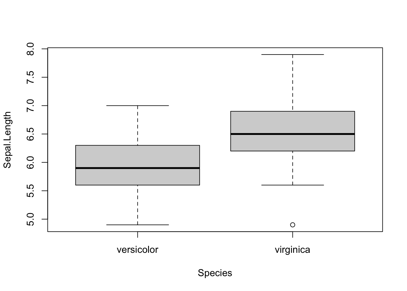
I thus wrote a piece of code that automated the process, by drawing boxplots and performing the tests on several variables at once. Below is the code I used, illustrating the process with the iris dataset. The Species variable has 3 levels, so let’s remove one, and then draw a boxplot and apply a t-test on all 4 continuous variables at once. Note that the continuous variables that we would like to test are variables 1 to 4 in the iris dataset.
dat <- iris

# remove one level to have only two groups
dat <- subset(dat, Species != "setosa")
dat$Species <- factor(dat$Species)

# boxplots and t-tests for the 4 variables at once
for (i in 1:4) { # variables to compare are variables 1 to 4
  boxplot(dat[, i] ~ dat$Species, # draw boxplots by group
    ylab = names(dat[i]), # rename y-axis with variable's name
    xlab = "Species"
  )
  print(t.test(dat[, i] ~ dat$Species)) # print results of t-test
}
##
## 	Welch Two Sample t-test
##
## data:  dat[, i] by dat$Species
## t = -5.6292, df = 94.025, p-value = 1.866e-07
## alternative hypothesis: true difference in means between group versicolor and group virginica is not equal to 0
## 95 percent confidence interval:
##  -0.8819731 -0.4220269
## sample estimates:
## mean in group versicolor  mean in group virginica
##                    5.936                    6.588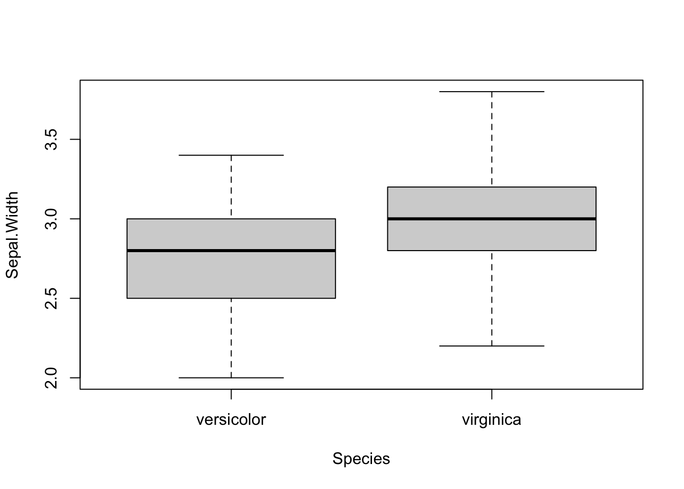
##
## 	Welch Two Sample t-test
##
## data:  dat[, i] by dat$Species
## t = -3.2058, df = 97.927, p-value = 0.001819
## alternative hypothesis: true difference in means between group versicolor and group virginica is not equal to 0
## 95 percent confidence interval:
##  -0.33028364 -0.07771636
## sample estimates:
## mean in group versicolor  mean in group virginica
##                    2.770                    2.974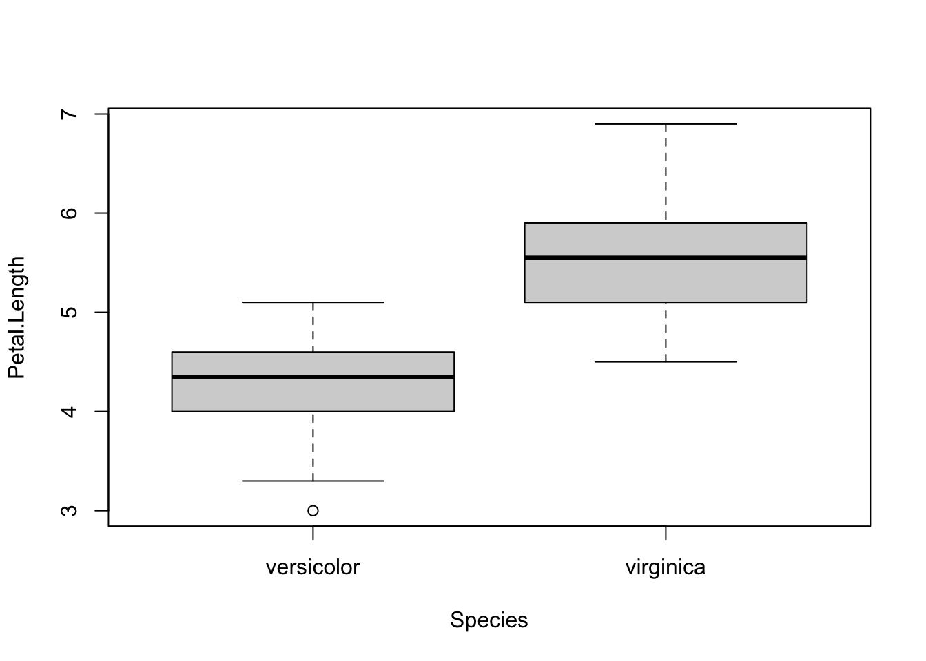
##
## 	Welch Two Sample t-test
##
## data:  dat[, i] by dat$Species
## t = -12.604, df = 95.57, p-value < 2.2e-16
## alternative hypothesis: true difference in means between group versicolor and group virginica is not equal to 0
## 95 percent confidence interval:
##  -1.49549 -1.08851
## sample estimates:
## mean in group versicolor  mean in group virginica
##                    4.260                    5.552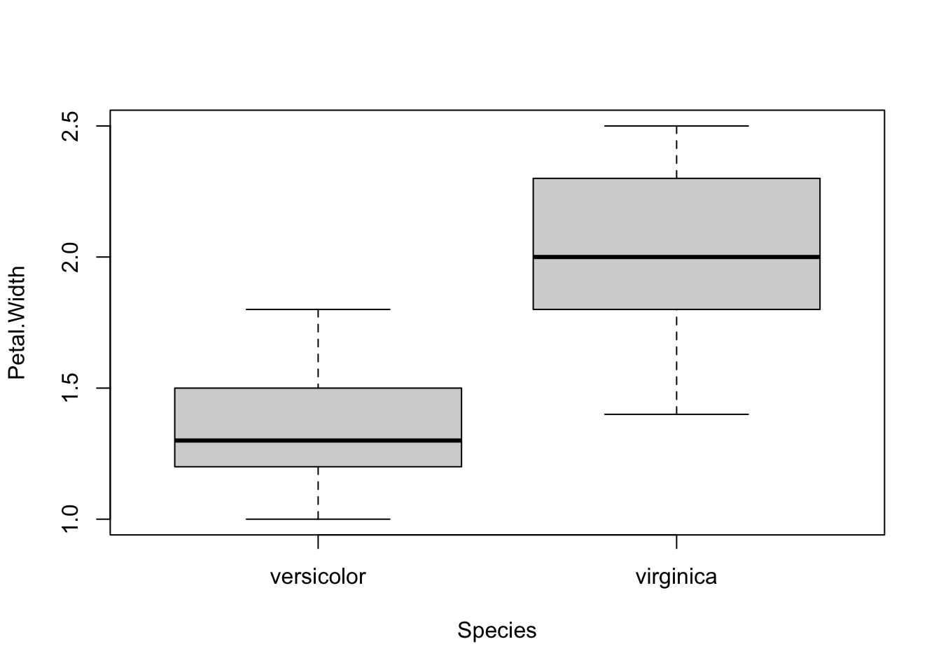
##
## 	Welch Two Sample t-test
##
## data:  dat[, i] by dat$Species
## t = -14.625, df = 89.043, p-value < 2.2e-16
## alternative hypothesis: true difference in means between group versicolor and group virginica is not equal to 0
## 95 percent confidence interval:
##  -0.7951002 -0.6048998
## sample estimates:
## mean in group versicolor  mean in group virginica
##                    1.326                    2.026
As you can see, the above piece of code draws a boxplot and then prints results of the test for each continuous variable, all at once.
At some point in the past, I even wrote code to:
- draw a boxplot
- test for the equality of variances (thanks to the Levene’s test)
- depending on whether the variances were equal or unequal, the appropriate test was applied: the Welch test if the variances were unequal and the Student’s t-test in the case the variances were equal (see more details about the different versions of the t-test for two samples)
- apply steps 1 to 3 for all continuous variables at once
I had a similar code for ANOVA in case I needed to compare more than two groups.
The code was doing the job relatively well. Indeed, thanks to this code I was able to test several variables in an automated way in the sense that it compared groups for all variables at once.
The only thing I had to change from one project to another is that I needed to modify the name of the grouping variable and the numbering of the continuous variables to test (Species and 1:4 in the above code).
Concise and easily interpretable results
T-test
Although it was working quite well and applicable to different projects with only minor changes, I was still unsatisfied with another point.
Someone who is proficient in statistics and R can read and interpret the output of a t-test without any difficulty. However, as you may have noticed with your own statistical projects, most people do not know what to look for in the results and are sometimes a bit confused when they see so many graphs, code, output, results and numeric values in a document. They are quite easily overwhelmed by this mass of information and unable to extract the key message.
With my old R routine, the time I was saving by automating the process of t-tests and ANOVA was (partially) lost when I had to explain R outputs to my students so that they could interpret the results correctly. Although most of the time it simply boiled down to pointing out what to look for in the outputs (i.e., p-values), I was still losing quite a lot of time because these outputs were, in my opinion, too detailed for most real-life applications and for students in introductory classes. In other words, too much information seemed to be confusing for many people so I was still not convinced that it was the most optimal way to share statistical results to nonscientists.
Of course, they came to me for statistical advices, so they expected to have these results and I needed to give them answers to their questions and hypotheses. Nonetheless, I wanted to find a better way to communicate these results to this type of audience, with the minimum of information required to arrive at a conclusion. No more and no less than that.
After a long time spent online trying to figure out a way to present results in a more concise and readable way, I discovered the {ggpubr} package. This package allows to indicate the test used and the p-value of the test directly on a ggplot2-based graph. It also facilitates the creation of publication-ready plots for non-advanced statistical audiences.
After many refinements and modifications of the initial code (available in this article), I finally came up with a rather stable and robust process to perform t-tests and ANOVA for more than one variable at once, and more importantly, make the results concise and easily readable by anyone (statisticians or not).
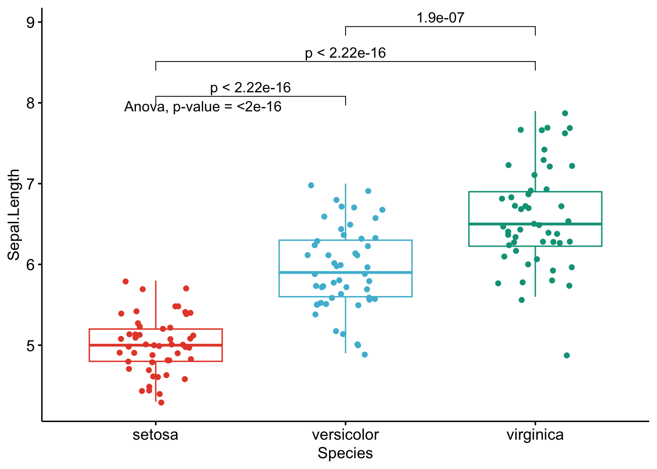
A graph is worth a thousand words, so here are the exact same tests than in the previous section, but this time with my new R routine:
library(ggpubr)

# Edit from here #
x <- which(names(dat) == "Species") # name of grouping variable
y <- which(names(dat) == "Sepal.Length" # names of variables to test
| names(dat) == "Sepal.Width" |
  names(dat) == "Petal.Length" |
  names(dat) == "Petal.Width")
method <- "t.test" # one of "wilcox.test" or "t.test"
paired <- FALSE # if paired make sure that in the dataframe you have first all individuals at T1, then all individuals again at T2
# Edit until here


# Edit at your own risk
for (i in y) {
  for (j in x) {
    if (paired == TRUE) {
      p <- ggpaired(dat,
        x = colnames(dat[j]), y = colnames(dat[i]),
        color = colnames(dat[j]), line.color = "gray", line.size = 0.4,
        palette = "npg",
        legend = "none",
        xlab = colnames(dat[j]),
        ylab = colnames(dat[i]),
        add = "jitter"
      )
    } else {
      p <- ggboxplot(dat,
        x = colnames(dat[j]), y = colnames(dat[i]),
        color = colnames(dat[j]),
        palette = "npg",
        legend = "none",
        add = "jitter"
      )
    }
    #  Add p-value
    print(p + stat_compare_means(aes(label = paste0(after_stat(method), ", p-value = ", after_stat(p.format))),
      method = method,
      paired = paired,
      # group.by = NULL,
      ref.group = NULL
    ))
  }
}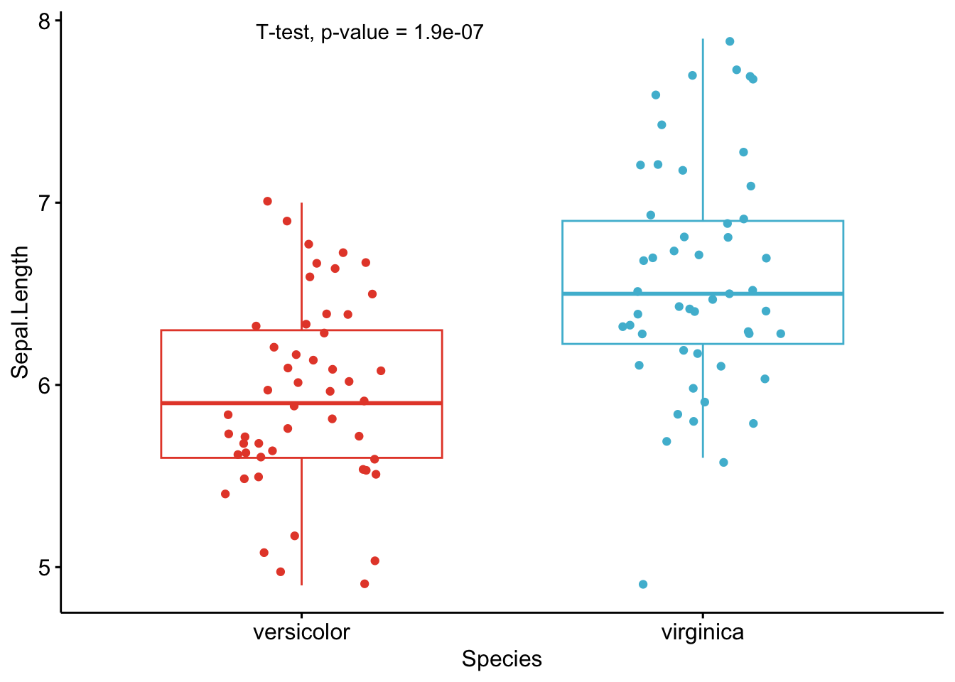
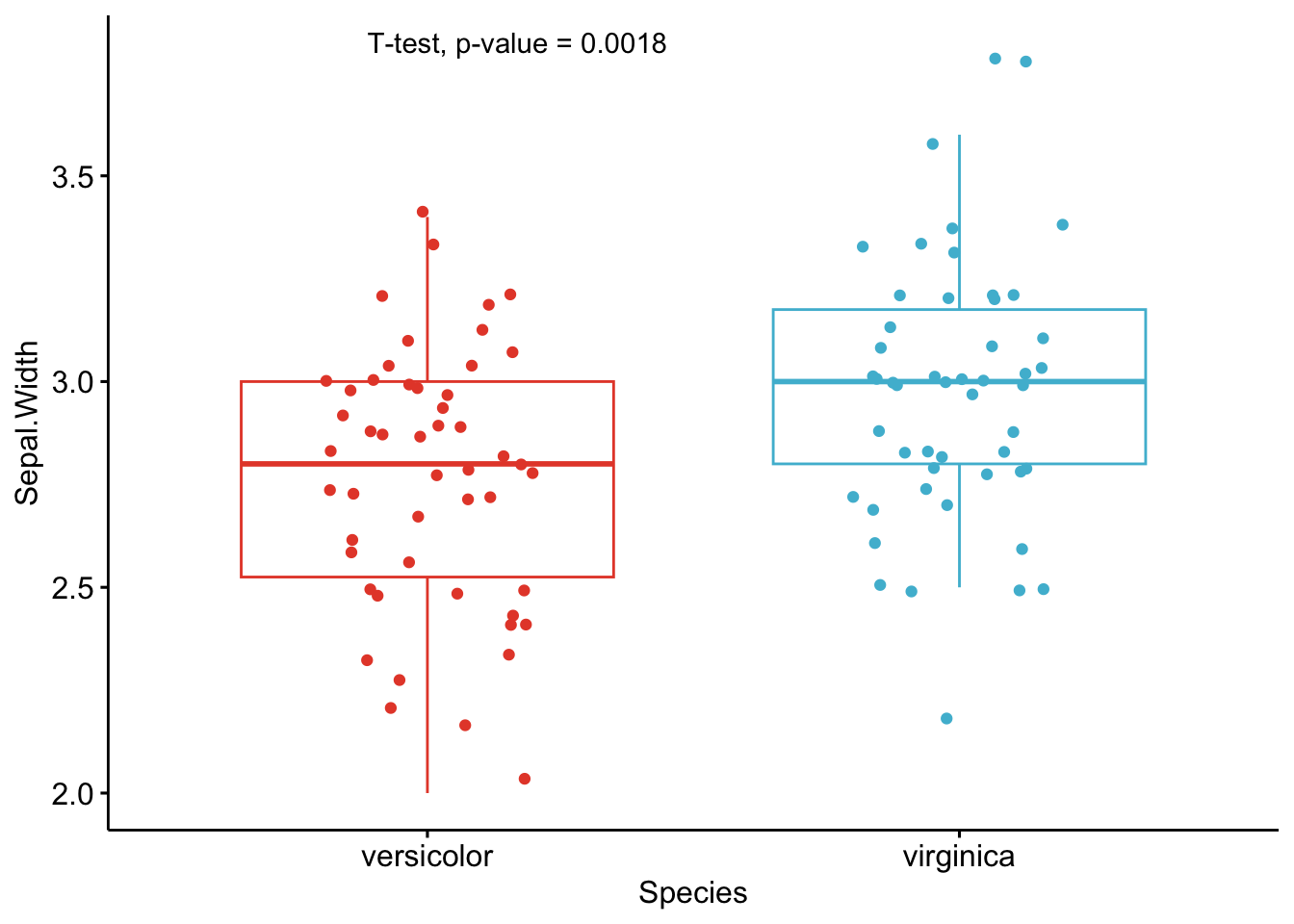
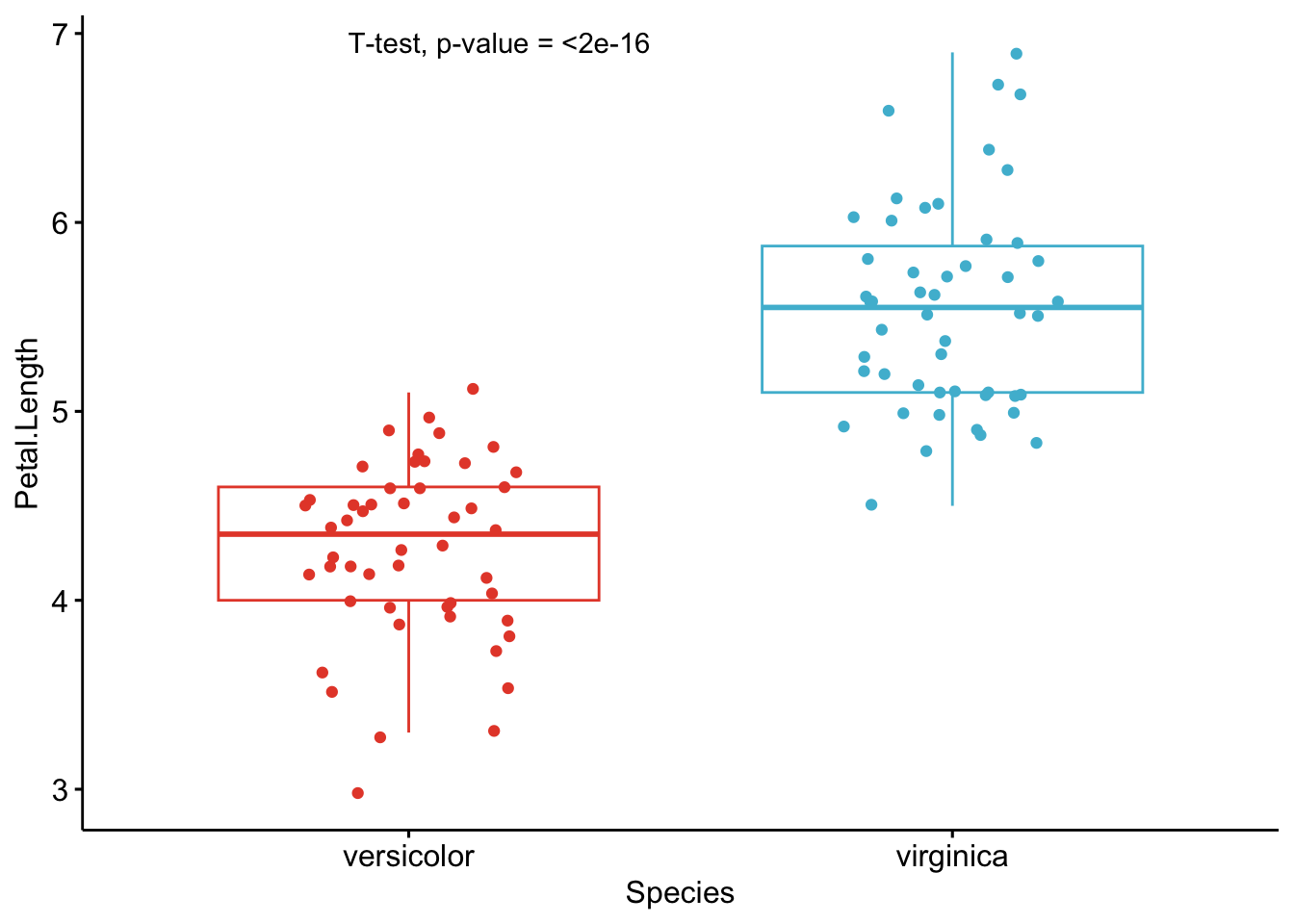
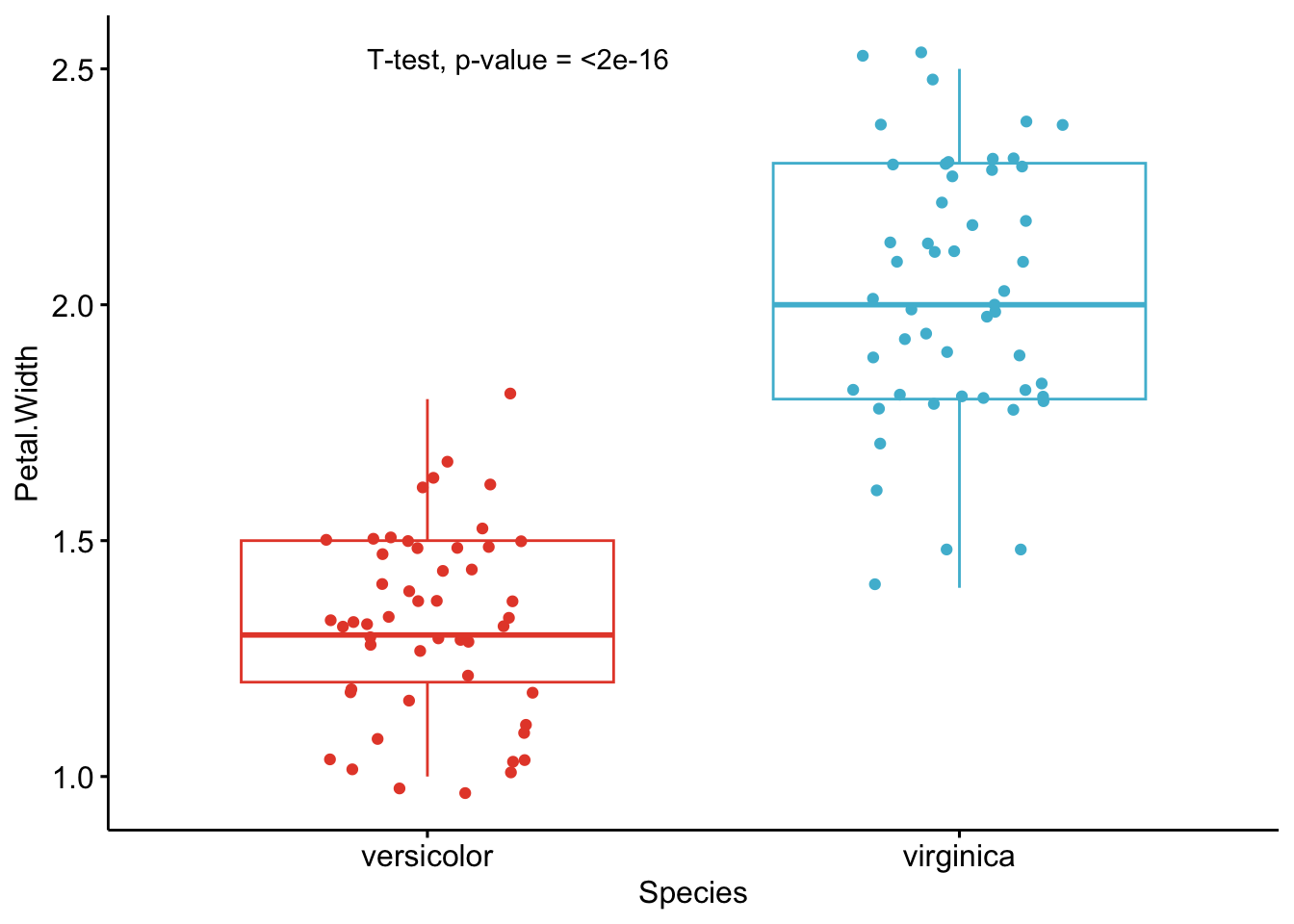
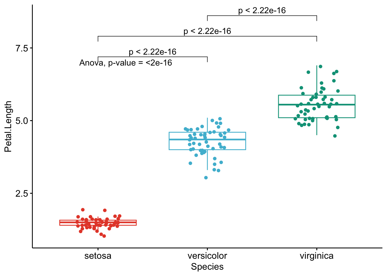
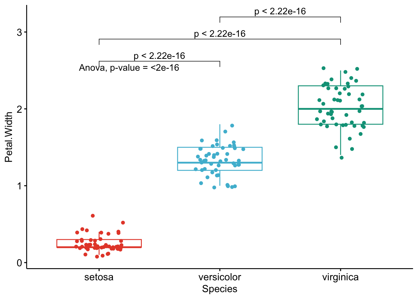
As you can see from the graphs above, only the most important information is presented for each variable:
- a visual comparison of the groups thanks to boxplots
- the name of the statistical test
- the p-value of the test
Of course, experts may be interested in more advanced results. However, this simple yet complete graph, which includes the name of the test and the p-value, gives all the necessary information to answer the question: “Are the groups different?”.
In my experience, I have noticed that students and professionals (especially those from a less scientific background) understand way better these results than the ones presented in the previous section.
The only lines of code that need to be modified for your own project is the name of the grouping variable (Species in the above code), the names of the variables you want to test (Sepal.Length, Sepal.Width, etc.),2 whether you want to apply a t-test (t.test) or Wilcoxon test (wilcox.test) and whether the samples are paired or not (FALSE if samples are independent, TRUE if they are paired).
Based on these graphs, it is easy, even for non-experts, to interpret the results and conclude that the versicolor and virginica species are significantly different in terms of all 4 variables (since all p-values \(< \frac{0.05}{4} = 0.0125\) (remind that the Bonferroni correction is applied to avoid the issue of multiple testing, so we divide the usual \(\alpha\) level by 4 because there are 4 t-tests)).
Additional p-value adjustment methods
If you would like to use another p-value adjustment method, you can use the p.adjust() function. Below are the raw p-values found above, together with p-values derived from the main adjustment methods (presented in a dataframe):
raw_pvalue <- numeric(length = length(1:4))
for (i in (1:4)) {
  raw_pvalue[i] <- t.test(dat[, i] ~ dat$Species,
    alternative = "two.sided"
  )$p.value
}

df <- data.frame(
  Variable = names(dat[, 1:4]),
  raw_pvalue = round(raw_pvalue, 3)
)

df$Bonferroni <-
  p.adjust(df$raw_pvalue,
    method = "bonferroni"
  )
df$BH <-
  p.adjust(df$raw_pvalue,
    method = "BH"
  )
df$Holm <-
  p.adjust(df$raw_pvalue,
    method = "holm"
  )
df$Hochberg <-
  p.adjust(df$raw_pvalue,
    method = "hochberg"
  )
df$Hommel <-
  p.adjust(df$raw_pvalue,
    method = "hommel"
  )
df$BY <-
  round(p.adjust(df$raw_pvalue,
    method = "BY"
  ), 3)
df
## Variable raw_pvalue Bonferroni BH Holm Hochberg Hommel BY
## 1 Sepal.Length 0.000 0.000 0.000 0.000 0.000 0.000 0.000
## 2 Sepal.Width 0.002 0.008 0.002 0.002 0.002 0.002 0.004
## 3 Petal.Length 0.000 0.000 0.000 0.000 0.000 0.000 0.000
## 4 Petal.Width 0.000 0.000 0.000 0.000 0.000 0.000 0.000Regardless of the p-value adjustment method, the two species are different for all 4 variables. Note that the adjustment method should be chosen before looking at the results to avoid choosing the method based on the results.
Below another function that allows to perform multiple Student’s t-tests or Wilcoxon tests at once and choose the p-value adjustment method. The function also allows to specify whether samples are paired or unpaired and whether the variances are assumed to be equal or not. (The code has been adapted from Mark White’s article.)
t_table <- function(data, dvs, iv,
                    var_equal = TRUE,
                    p_adj = "none",
                    alpha = 0.05,
                    paired = FALSE,
                    wilcoxon = FALSE) {
  if (!inherits(data, "data.frame")) {
    stop("data must be a data.frame")
  }

  if (!all(c(dvs, iv) %in% names(data))) {
    stop("at least one column given in dvs and iv are not in the data")
  }

  if (!all(sapply(data[, dvs], is.numeric))) {
    stop("all dvs must be numeric")
  }

  if (length(unique(na.omit(data[[iv]]))) != 2) {
    stop("independent variable must only have two unique values")
  }

  out <- lapply(dvs, function(x) {
    if (paired == FALSE & wilcoxon == FALSE) {
      tres <- t.test(data[[x]] ~ data[[iv]], var.equal = var_equal)
    } else if (paired == FALSE & wilcoxon == TRUE) {
      tres <- wilcox.test(data[[x]] ~ data[[iv]])
    } else if (paired == TRUE & wilcoxon == FALSE) {
      tres <- t.test(data[[x]] ~ data[[iv]],
        var.equal = var_equal,
        paired = TRUE
      )
    } else {
      tres <- wilcox.test(data[[x]] ~ data[[iv]],
        paired = TRUE
      )
    }

    c(
      p_value = tres$p.value
    )
  })

  out <- as.data.frame(do.call(rbind, out))
  out <- cbind(variable = dvs, out)
  names(out) <- gsub("[^0-9A-Za-z_]", "", names(out))

  out$p_value <- p.adjust(out$p_value, p_adj)
  out$conclusion <- ifelse(out$p_value < alpha,
    paste0("Reject H0 at ", alpha * 100, "%"),
    paste0("Do not reject H0 at ", alpha * 100, "%")
  )
  out$p_value <- ifelse(out$p_value < 0.001,
    "<0.001",
    round(out$p_value, 3)
  )

  return(out)
}
Applied to our dataset, with no adjustment method for the p-values:
result <- t_table(
  data = dat,
  c("Sepal.Length", "Sepal.Width", "Petal.Length", "Petal.Width"),
  "Species"
)

result
## variable p_value conclusion
## 1 Sepal.Length <0.001 Reject H0 at 5%
## 2 Sepal.Width 0.002 Reject H0 at 5%
## 3 Petal.Length <0.001 Reject H0 at 5%
## 4 Petal.Width <0.001 Reject H0 at 5%And with the Holm (1979) adjustment method:
result <- t_table(
  data = dat,
  c("Sepal.Length", "Sepal.Width", "Petal.Length", "Petal.Width"),
  "Species",
  p_adj = "holm"
)

result
## variable p_value conclusion
## 1 Sepal.Length <0.001 Reject H0 at 5%
## 2 Sepal.Width 0.002 Reject H0 at 5%
## 3 Petal.Length <0.001 Reject H0 at 5%
## 4 Petal.Width <0.001 Reject H0 at 5%Again, with the Holm’s adjustment method, we conclude that, at the 5% significance level, the two species are significantly different from each other in terms of all 4 variables.
ANOVA
Below the same process with an ANOVA. Note that we reload the dataset iris to include all three Species this time:
dat <- iris

# Edit from here
x <- which(names(dat) == "Species") # name of grouping variable
y <- which(names(dat) == "Sepal.Length" # names of variables to test
| names(dat) == "Sepal.Width" |
  names(dat) == "Petal.Length" |
  names(dat) == "Petal.Width")
method1 <- "anova" # one of "anova" or "kruskal.test"
method2 <- "t.test" # one of "wilcox.test" or "t.test"
my_comparisons <- list(c("setosa", "versicolor"), c("setosa", "virginica"), c("versicolor", "virginica")) # comparisons for post-hoc tests
# Edit until here


# Edit at your own risk
for (i in y) {
  for (j in x) {
    p <- ggboxplot(dat,
      x = colnames(dat[j]), y = colnames(dat[i]),
      color = colnames(dat[j]),
      legend = "none",
      palette = "npg",
      add = "jitter"
    )
    print(
      p + stat_compare_means(aes(label = paste0(after_stat(method), ", p-value = ", after_stat(p.format))),
        method = method1, label.y = max(dat[, i], na.rm = TRUE)
      )
      + stat_compare_means(comparisons = my_comparisons, method = method2, label = "p.format") # remove if p-value of ANOVA or Kruskal-Wallis test >= alpha
    )
  }
}

Like the improved routine for the t-test, I have noticed that students and non-expert professionals understand ANOVA results presented this way much more easily compared to the default R outputs.
With one graph for each variable, it is easy to see that all species are different from each other in terms of all 4 variables.3
If you want to apply the same automated process to your data, you will need to modify the name of the grouping variable (Species), the names of the variables you want to test (Sepal.Length, etc.), whether you want to perform an ANOVA (anova) or Kruskal-Wallis test (kruskal.test) and finally specify the comparisons for the post-hoc tests.4
To go even further
As we have seen, these two improved R routines allow to:
- Perform t-tests and ANOVA on a small or large number of variables with only minor changes to the code. I basically only have to replace the variable names and the name of the test I want to use. It takes almost the same time to test one or several variables so it is quite an improvement compared to testing one variable at a time.
- Share test results in a much proper and cleaner way. This is possible thanks to a graph showing the observations by group and the p-value of the appropriate test included directly on the graph. This is particularly important when communicating results to a wider audience or to people from diverse backgrounds.
However, like most of my R routines, these two pieces of code are still a work in progress. Below are some additional features I have been thinking of and which could be added in the future to make the process of comparing two or more groups even more optimal:
- Add the possibility to select variables by their numbering in the dataframe. For the moment it is only possible to do it via their names. This will allow to automate the process even further because instead of typing all variable names one by one, we could simply type
4:25(to test variables 4 to 25 for instance). - Add the possibility to choose a p-value adjustment method. Currently, raw p-values are displayed in the graphs and I manually adjust them afterwards or adjust the \(\alpha\).
- When comparing more than two groups, it is only possible to apply an ANOVA or Kruskal-Wallis test at the moment. A major improvement would be to add the possibility to perform a repeated measures ANOVA (i.e., an ANOVA when the samples are dependent). It is currently already possible to do a t-test with two paired samples, but it is not yet possible to do the same with more than two groups.
- Another less important (yet still nice) feature when comparing more than 2 groups would be to automatically apply post-hoc tests only in the case where the null hypothesis of the ANOVA or Kruskal-Wallis test is rejected (so when there is at least one group different from the others, because if the null hypothesis of equal groups is not rejected we do not apply a post-hoc test). At the present time, I manually add or remove the code that displays the p-values of post-hoc tests depending on the global p-value of the ANOVA or Kruskal-Wallis test.
I will try to add these features in the future, or I would be glad to help if the author of the {ggpubr} package needs help in including these features (I hope he will see this article!).
Last but not least, the following packages may be of interest to some readers:
- If you want to report statistical results on a graph, I advise you to check the
{ggstatsplot}package and in particular theggbetweenstats()andggwithinstats()functions. These functions allow to compare a continuous variable across multiple groups or conditions (for both independent and paired samples). Two advantages of the functions is that:- it is very easy to switch from parametric to nonparametric tests and
- it automatically runs an ANOVA or t-test depending on the number of groups to compare
Note that many different statistical results are displayed on the graph, not only the name of the test and the p-value so a bit of simplicity and clarity is lost for more precision. However, it is still very convenient to be able to include tests results on a graph in order to combine the advantages of a visualization and a sound statistical analysis. Something that I still need to figure out is how to run the code on several variables at once.
- The
{compareGroups}package also provides a nice way to compare groups. It comes with a really complete Shiny app, available with:
# install.packages("compareGroups")
library(compareGroups)
cGroupsWUI()
Update with the {ggstatsplot} package
Several months after having written this article, I finally found a way to plot and run analyses on several variables at once with the package {ggstatsplot} (Patil 2021). This was the main feature I was missing and which prevented me from using it more often.
Although I still find that too much statistical details are displayed (in particular for non experts), I still believe the ggbetweenstats() and ggwithinstats() functions are worth mentioning in this article. I actually now use those two functions almost as often as my previous routines because:
- I do not have to care about the number of groups to compare, the functions automatically choose the appropriate test according to the number of groups (ANOVA for 3 groups or more, and t-test for 2 groups)
- I can select variables based on their column numbering, and not based on their names anymore (which prevents me from writing those variable names manually)
- When comparing 3 or more groups (so for ANOVA, Kruskal-Wallis, repeated measure ANOVA or Friedman), \(p\)-values of the post-hoc tests within each dependent variable are by default the adjusted \(p\)-values (Holm is the default but many adjustment methods are available)
- It is possible to compare both independent and paired samples, no matter the number of groups (remember that with the
ggpubrpackage I could only do paired samples for two samples, not for 3 samples) - They allow to easily switch between the parametric and nonparametric version
- All this in a more concise manner using the
{purrr}package
For those of you who are interested, below my updated R routine which include these functions and applied this time on the penguins dataset.
library(palmerpenguins)

dat <- penguins
str(dat)
## tibble [344 × 8] (S3: tbl_df/tbl/data.frame)
## $ species : Factor w/ 3 levels "Adelie","Chinstrap",..: 1 1 1 1 1 1 1 1 1 1 ...
## $ island : Factor w/ 3 levels "Biscoe","Dream",..: 3 3 3 3 3 3 3 3 3 3 ...
## $ bill_length_mm : num [1:344] 39.1 39.5 40.3 NA 36.7 39.3 38.9 39.2 34.1 42 ...
## $ bill_depth_mm : num [1:344] 18.7 17.4 18 NA 19.3 20.6 17.8 19.6 18.1 20.2 ...
## $ flipper_length_mm: int [1:344] 181 186 195 NA 193 190 181 195 193 190 ...
## $ body_mass_g : int [1:344] 3750 3800 3250 NA 3450 3650 3625 4675 3475 4250 ...
## $ sex : Factor w/ 2 levels "female","male": 2 1 1 NA 1 2 1 2 NA NA ...
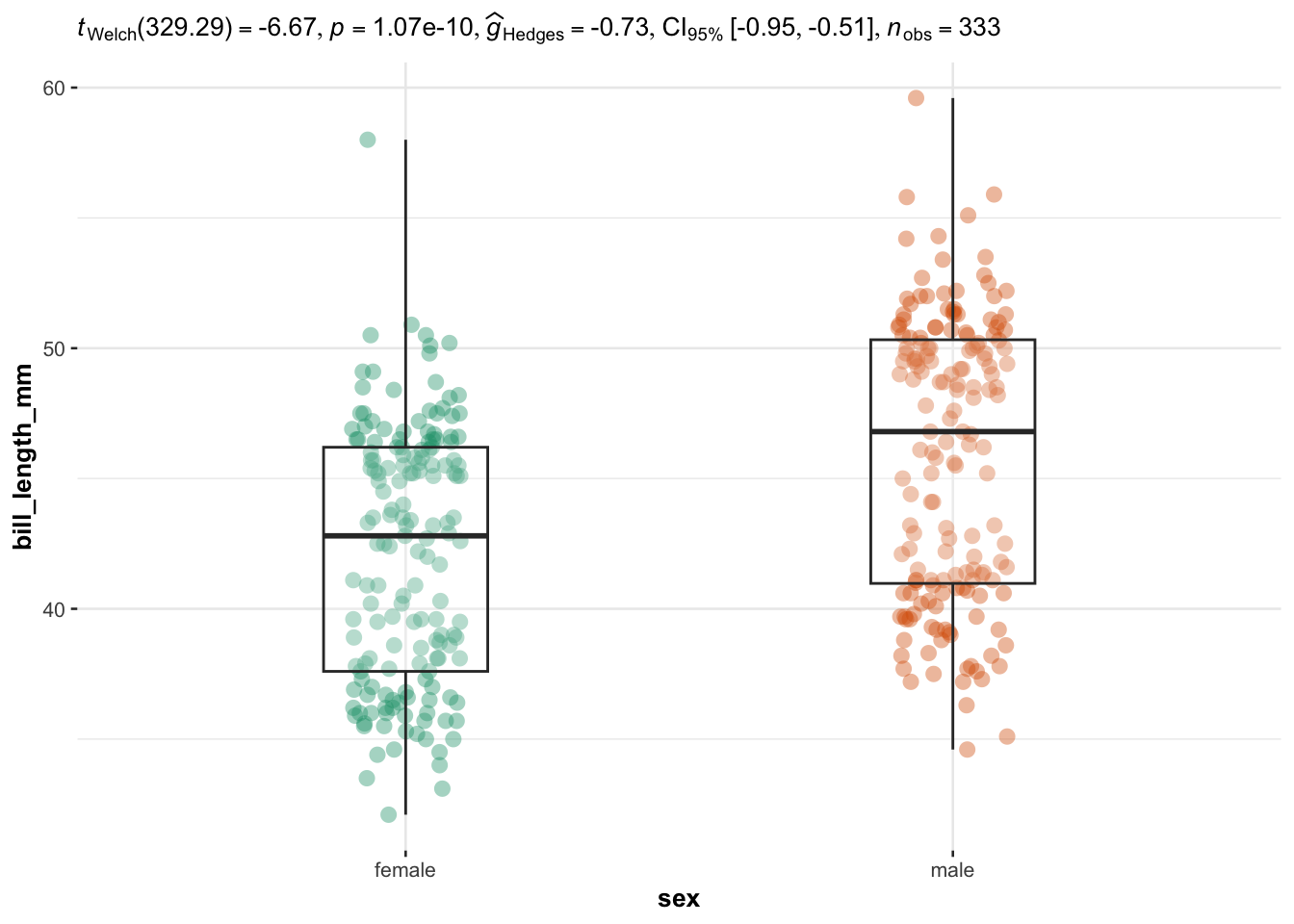
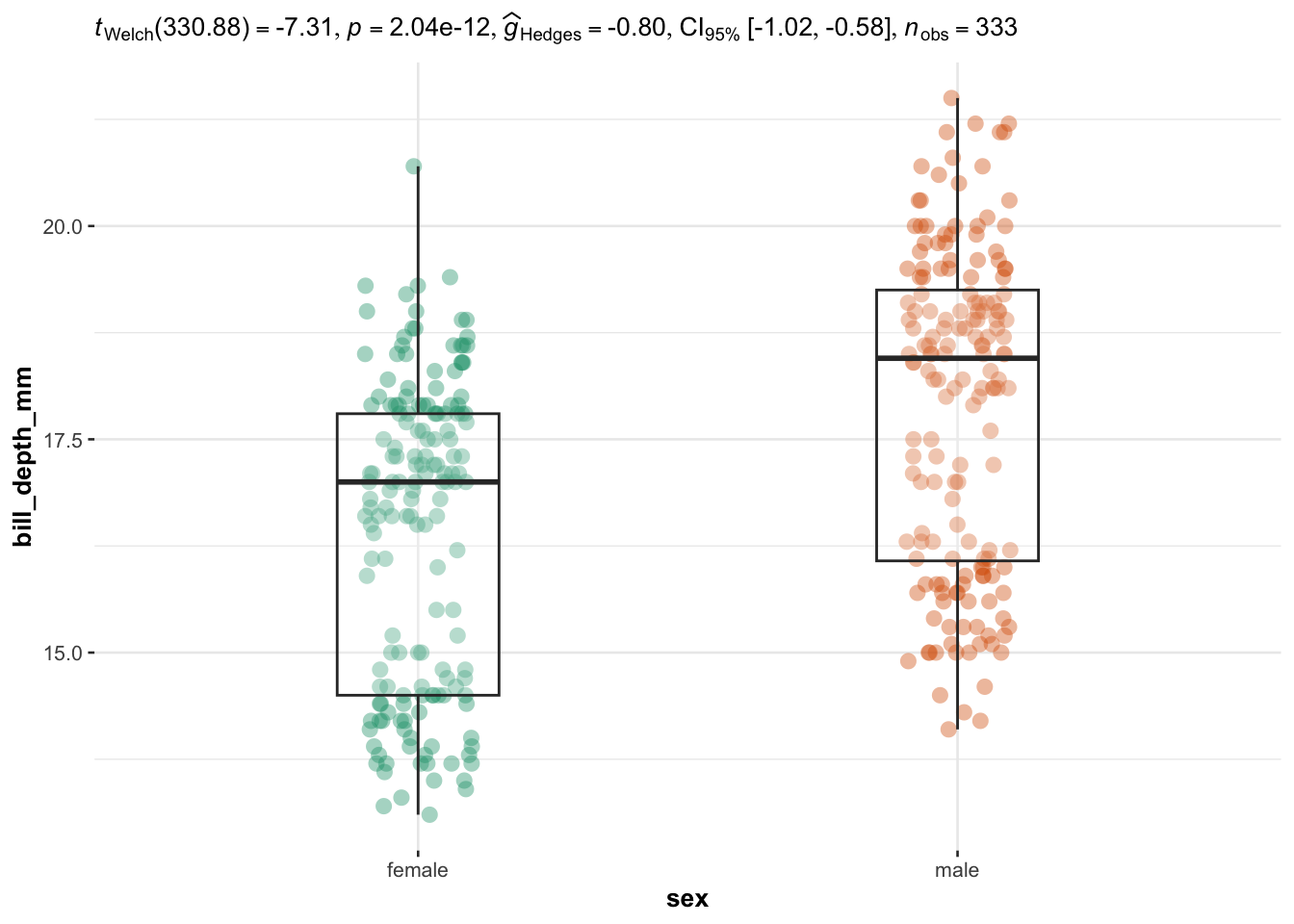
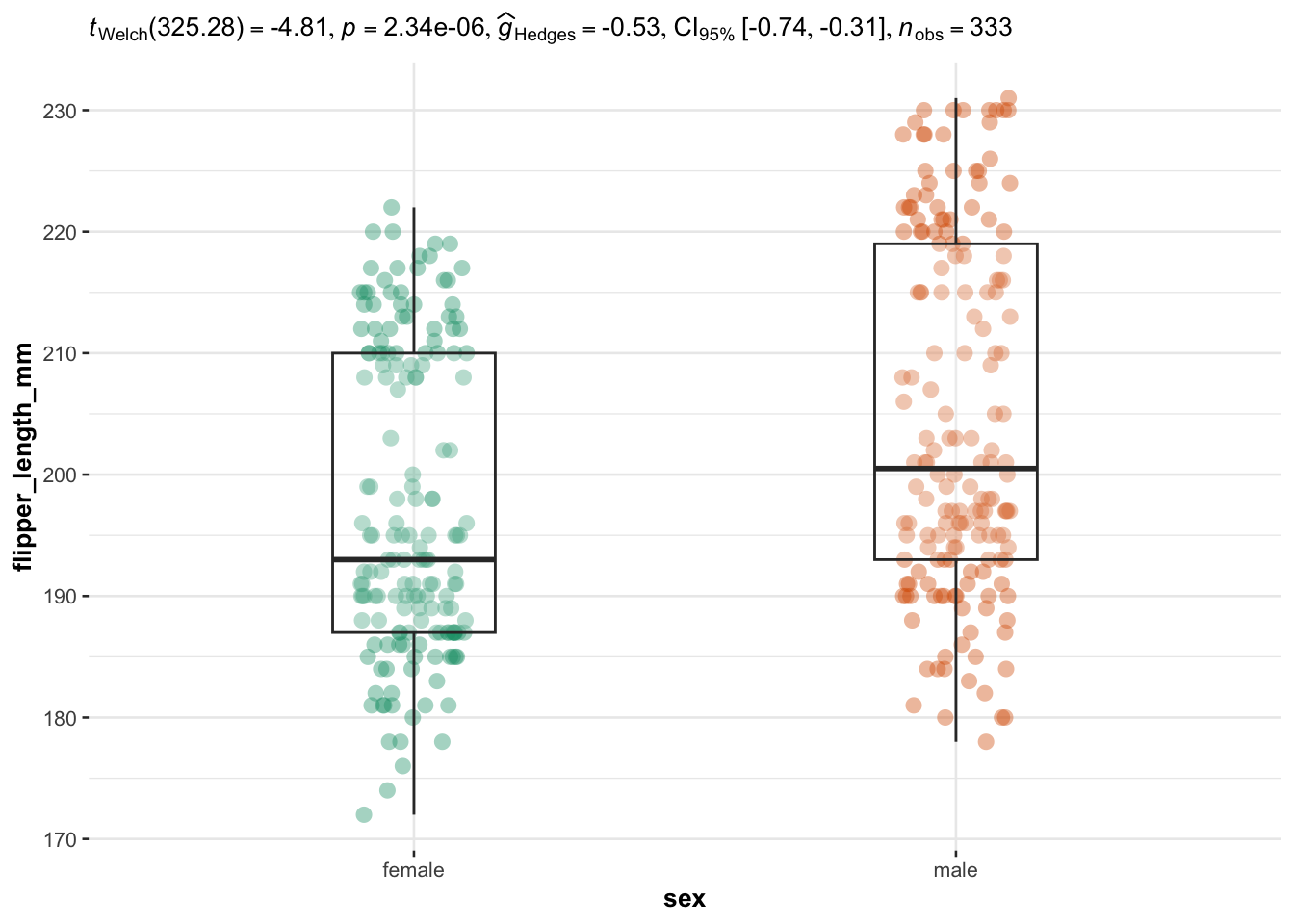
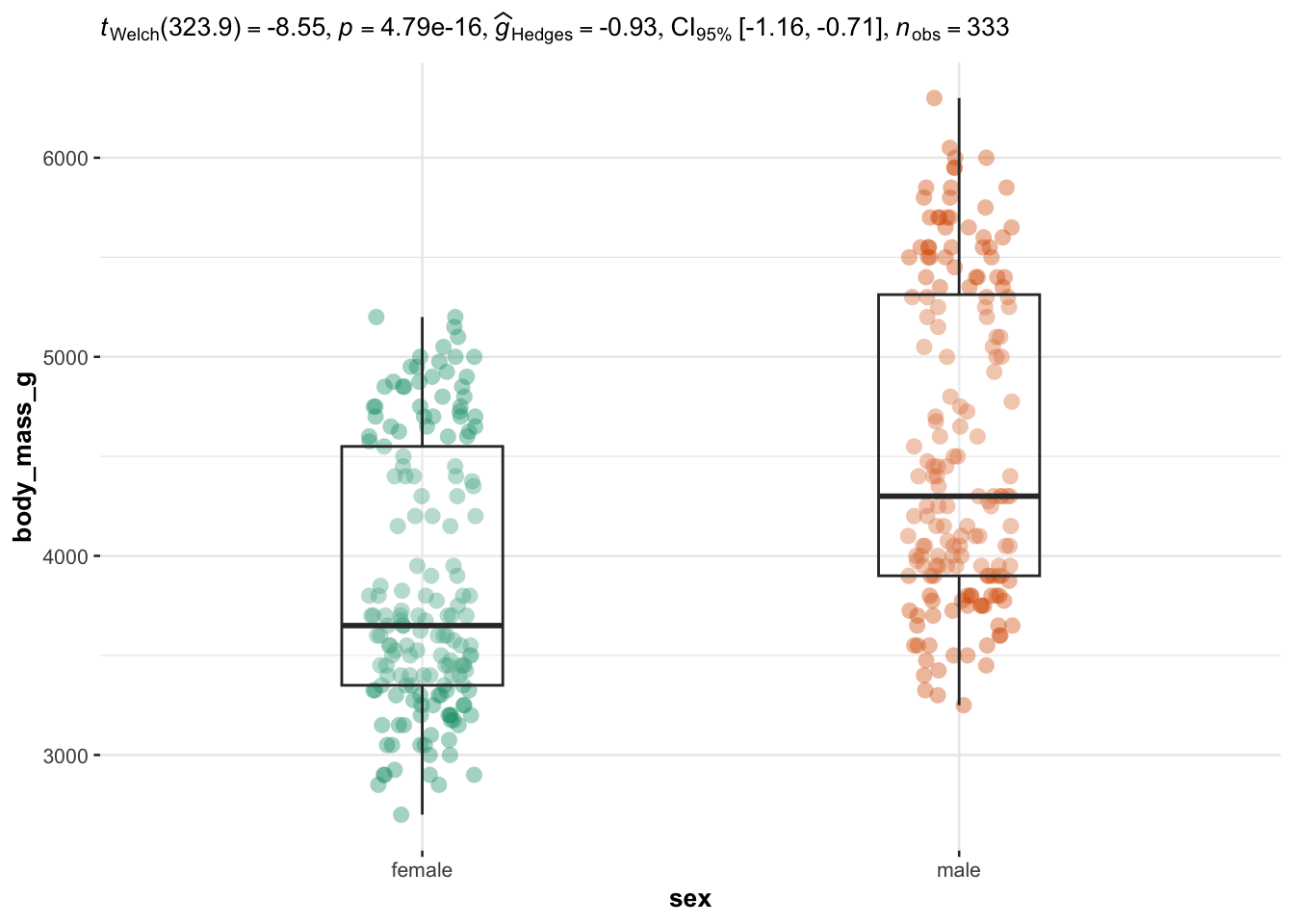
## $ year : int [1:344] 2007 2007 2007 2007 2007 2007 2007 2007 2007 2007 ...We illustrate the routine for two groups with the variables sex (two factors) as independent variable, and the 4 quantitative continuous variables bill_length_mm, bill_depth_mm, flipper_length_mm and body_mass_g as dependent variables:
library(ggstatsplot)
library(tibble)

# Comparison between sexes

# edit from here
x <- "sex"
cols <- 3:6 # the 4 continuous dependent variables
type <- "parametric" # given the large number of observations, we use the parametric version
paired <- FALSE # FALSE for independent samples, TRUE for paired samples
# edit until here

# edit at your own risk
plotlist <-
  purrr::pmap(
    .l = list(
      data = list(as_tibble(dat)),
      x = x,
      y = as.list(colnames(dat)[cols]),
      plot.type = "box", # for boxplot
      type = type, # parametric or nonparametric
      pairwise.comparisons = TRUE, # to run post-hoc tests if more than 2 groups
      pairwise.display = "significant", # show only significant differences
      bf.message = FALSE, # remove message about Bayes Factor
      centrality.plotting = FALSE # remove central measure
    ),
    .f = ifelse(paired, # automatically use ggwithinstats if paired samples, ggbetweenstats otherwise
      ggstatsplot::ggwithinstats,
      ggstatsplot::ggbetweenstats
    ),
    violin.args = list(width = 0, linewidth = 0) # remove violin plots and keep only boxplots
  )

# print all plots together with statistical results
for (i in 1:length(plotlist)) {
  print(plotlist[[i]])
}
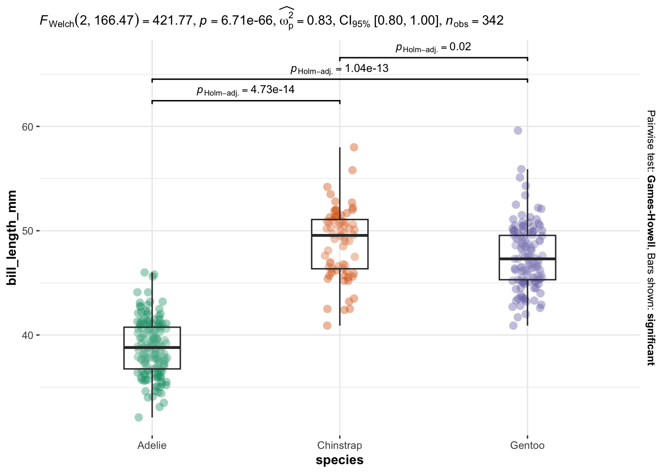
We now illustrate the routine for 3 groups or more with the variable species (three factors) as independent variable, and the 4 same dependent variables:
# Comparison between species

# edit from here
x <- "species"
cols <- 3:6 # the 4 continuous dependent variables
type <- "parametric" # given the large number of observations, we use the parametric version
paired <- FALSE # FALSE for independent samples, TRUE for paired samples
# edit until here

# edit at your own risk
plotlist <-
  purrr::pmap(
    .l = list(
      data = list(as_tibble(dat)),
      x = x,
      y = as.list(colnames(dat)[cols]),
      plot.type = "box", # for boxplot
      type = type, # parametric or nonparametric
      pairwise.comparisons = TRUE, # to run post-hoc tests if more than 2 groups
      pairwise.display = "significant", # show only significant differences
      bf.message = FALSE, # remove message about Bayes Factor
      centrality.plotting = FALSE # remove central measure
    ),
    .f = ifelse(paired, # automatically use ggwithinstats if paired samples, ggbetweenstats otherwise
      ggstatsplot::ggwithinstats,
      ggstatsplot::ggbetweenstats
    ),
    violin.args = list(width = 0, linewidth = 0) # remove violin plots and keep only boxplots
  )

# print all plots together with statistical results
for (i in 1:length(plotlist)) {
  print(plotlist[[i]])
}
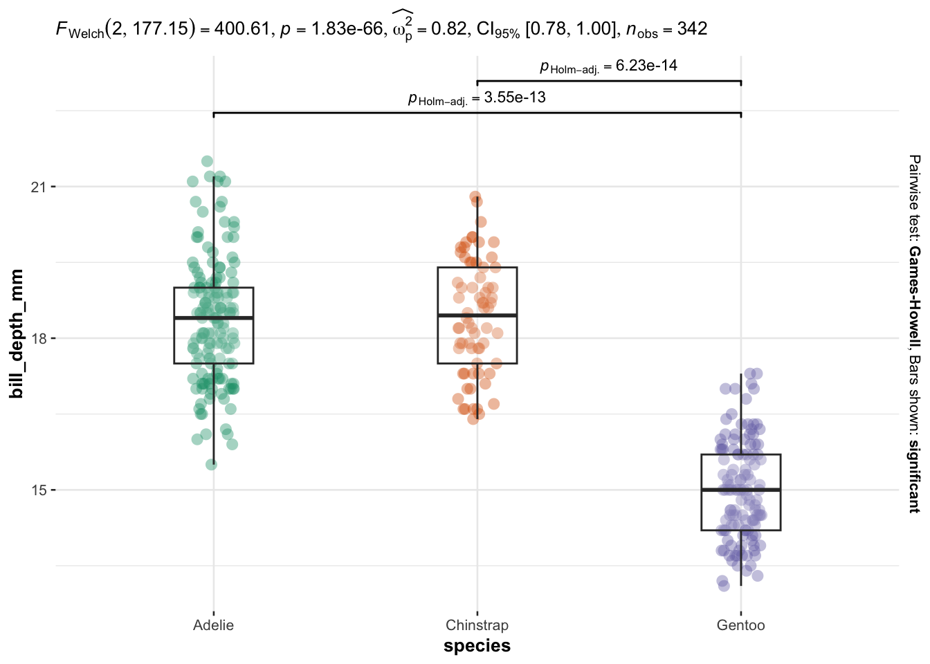
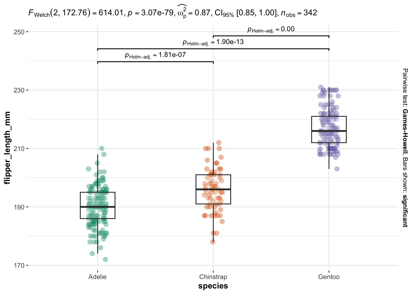
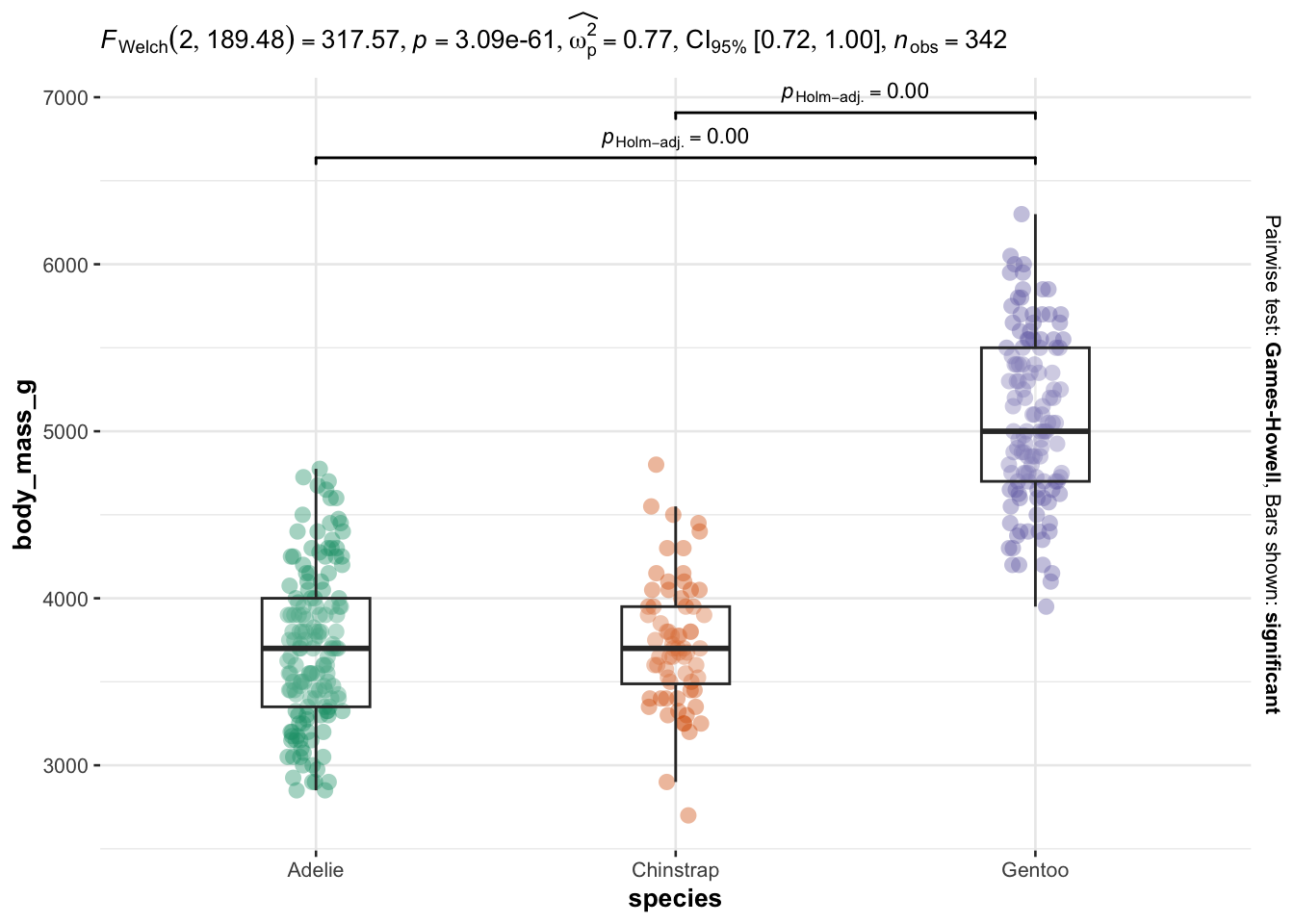
As you can see, I only have to specify:
- the name of the grouping variable (
sexandspecies), - the number of the dependent variables (variables 3 to 6 in the dataset),
- whether I want to use the parametric or nonparametric version and
- whether samples are independent (
paired = FALSE) or paired (paired = TRUE).
Everything else is automated—the outputs show a graphical representation of what we are comparing, together with the details of the statistical analyses in the subtitle of the plot (the \(p\)-value among others).
Note that the code shown above is actually the same if I want to compare 2 groups or more than 2 groups. I wrote twice the same code (once for 2 groups and once again for 3 groups) for illustrative purposes only, but they are the same and should be treated as one for your projects.
I must admit I am quite satisfied with this routine, now that:
- I can automate it on many variables at once and I do not need to write the variable names manually anymore,
- at the same time, I can choose the appropriate test among all the available ones (depending on the number of groups, whether they are paired or not, and whether I want to use the parametric or nonparametric version).
Nonetheless, I must also admit that I am still not satisfied with the level of details of the statistical results. As already mentioned, many students get confused and get lost in front of so much information (except the \(p\)-value and the number of observations, most of the details are rather obscure to them because they are not covered in introductory statistic classes).
I saved time thanks to all improvements in comparison to my previous routine, but I definitely lose time when I have to point out to them what they should look for. After discussing with other professors, I noticed that they have the same problem.
For the moment, you can only print all results or none. I have opened an issue kindly requesting to add the possibility to display only a summary (with the \(p\)-value and the name of the test for instance).5 I will update again this article if the maintainer of the package includes this feature in the future. So stay tuned!
Conclusion
Thanks for reading.
I hope this article will help you to perform t-tests and ANOVA for multiple variables at once and make the results more easily readable and interpretable by non-scientists. Learn more about the t-test to compare two groups, or the ANOVA to compare 3 groups or more.
As always, if you have a question or a suggestion related to the topic covered in this article, please add it as a comment so other readers can benefit from the discussion.
References
In theory, an ANOVA can also be used to compare two groups as it will give the same results compared to a Student’s t-test, but in practice we use the Student’s t-test to compare two groups and the ANOVA to compare three groups or more.↩︎
Do not forget to separate the variables you want to test with
|.↩︎Do not forget to adjust the \(p\)-values or the significance level \(\alpha\). If you use the Bonferroni correction, the adjusted \(\alpha\) is simply the desired \(\alpha\) level divided by the number of comparisons.↩︎
Post-hoc test is only the name used to refer to a specific type of statistical tests. Post-hoc test includes, among others, the Tukey HSD test, the Bonferroni correction, Dunnett’s test. Even if an ANOVA or a Kruskal-Wallis test can determine whether there is at least one group that is different from the others, it does not allow us to conclude which are different from each other. For this purpose, there are post-hoc tests that compare all groups two by two to determine which ones are different, after adjusting for multiple comparisons. Concretely, post-hoc tests are performed to each possible pair of groups after an ANOVA or a Kruskal-Wallis test has shown that there is at least one group which is different (hence “post” in the name of this type of test). The null and alternative hypotheses and the interpretations of these tests are similar to a Student’s t-test for two samples.↩︎
I am open to contribute to the package if I can help!↩︎
Liked this post?
- Get updates every time a new article is published (no spam and unsubscribe anytime)
- Support the blog
- Share on:


