
How to perform a one-sample t-test by hand and in R: test on one mean

Introduction
After having written an article on the Student’s t-test for two samples (independent and paired samples), I believe it is time to explain in details how to perform one-sample t-tests by hand and in R.
One-sample t-test is an important part of inferential statistics (probably one of the first statistical test that students learn). Remind that, unlike descriptive statistics, inferential statistics is a branch of statistics aiming at drawing conclusions about one or two populations, based on a subset (or two) of that population (called samples). In other words, we first collect a random set of observations from a population, and then some measurements are calculated in order to generalize to the population the information found through the sample.
In this context, the one-sample t-test is used to determine whether the mean of a measurement variable is different from a specified value (a belief or a theoretical expectation for example). It works as follows: if the mean of the sample is too distant from the specified value (the value under the null hypothesis), it is considered that the mean of the population is different from what is expected. On the contrary, if the mean of the sample is close to the specified value, we cannot reject the hypothesis that the population mean is equal to what is expected.
Like the Student’s t-test for two samples and the ANOVA (for 3 or more samples), there are also different versions of the one-sample t-test. Luckily, there are only two different versions for this test (the Student’s t-test for two samples has 5 versions!). The difference between the two versions of the one-sample t-test lies in the fact that one version is used when the variance of the population (not the variance of the sample!) is known, the other version being used when the variance of the population is unknown.
In this article, I will first detail step by step how to perform both versions of the one-sample t-test by hand. The analyses will be done on a small set of observations for the sake of illustration and easiness. I will then show how to perform this test in R with the exact same data in order to verify the results found by hand. Reminders about the reasoning behind hypothesis tests, interpretations of the p-value and the results, and assumptions of this test will also be presented.
Note that the aim of this article is to show how to compute the one-sample t-test by hand and in R, so we refrain from testing the assumptions and we assume all assumptions are met for this exercise. For completeness, we still mention the assumptions and how to test them. Interested readers are invited to have a look at the end of the article for more information about these assumptions.
Null and alternative hypothesis
Before diving into the computations of the one-sample t-test by hand, let’s recap the null and alternative hypotheses of this test:
- \(H_0\): \(\mu = \mu_0\)
- \(H_1\): \(\mu \ne \mu_0\)
where \(\mu\) is the population mean and \(\mu_0\) is the known or hypothesized value of the mean in the population.
This is in the general case where we simply want to determine whether the population mean is different (in terms of the dependent variable) compared to the hypothesized value. In this sense, we have no prior belief about the population mean being larger or smaller than the hypothesized value. This type of test is referred as a two-sided or bilateral test.
If we have some prior beliefs about the population mean being larger or smaller than the hypothesized value, the one-sample t-test also allows to test the following hypotheses:
- \(H_0\): \(\mu = \mu_0\)
- \(H_1\): \(\mu > \mu_0\)
or
- \(H_0\): \(\mu = \mu_0\)
- \(H_1\): \(\mu < \mu_0\)
In the first case, we want to test if the population mean is significantly larger than the hypothesized value, while in the latter case, we want to test if the population mean is significantly smaller than the hypothesized value. This type of test is referred as a one-sided or unilateral test.
Hypothesis testing
In statistics, many statistical tests is in the form of hypothesis tests. Hypothesis tests are used to determine whether a certain belief can be deemed as true (plausible) or not, based on the data at hand (i.e., the sample(s)). Most hypothesis tests boil down to the following 4 steps:1
- State the null and alternative hypothesis.
- Compute the test statistic, denoted t-stat. Formulas to compute the test statistic differ among the different versions of the one-sample t-test but they have the same structure. See scenarios 1 and 2 below to see the different formulas.
- Find the critical value given the theoretical statistical distribution of the test, the parameters of the distribution and the significance level \(\alpha\). For the two versions of the one-sample t-test, it is either the normal or the Student’s t distribution (t denoting the Student distribution and z denoting the normal distribution).
- Conclude by comparing the t-stat (found in step 2.) with the critical value (found in step. 3). If the t-stat lies in the rejection region (determined thanks to the critical value and the direction of the test), we reject the null hypothesis, otherwise we do not reject the null hypothesis. These two alternatives (reject or do not reject the null hypothesis) are the only two possible solutions, we never “accept” an hypothesis. It is also a good practice to always interpret the decision in the terms of the initial question.
For the interested reader, see these 4 steps of hypothesis testing in more details in this article.
Two versions of the one-sample t-test
There are two versions of the one-sample t-test, depending on whether the variance of the population (not the variance of the sample!) is known or unknown. This criteria is rather straightforward, we either know the variance of the population or we do not. The variance of the population cannot be computed because if you can compute the variance of a population, it means you have the data for the whole population, then there is no need to do a hypothesis test anymore…
So the variance of the population is either given in the statement (use them in that case), or there is no information about the variance and in that case, it is assumed that the variance is unknown. In practice, the variance of the population is most of the time unknown. However, we still illustrate how to do both versions of this test by hand and in R in the next sections following the 4 steps of a hypothesis test.
How to compute the one-sample t-test by hand?
Note that the data are artificial and do not represent any real variable. Furthermore, remind that the assumptions may or may not be met. The point of the article is to detail how to compute the different versions of the test by hand and in R, so all assumptions are assumed to be met. Moreover, we assume that for all tests the significance level, that is, the type I error is \(\alpha = 5\)%.
If you are interested in applying these tests by hand without having to do the computations yourself, here is a Shiny app which does it for you. You just need to enter the data and choose the appropriate version of the test thanks to the sidebar menu. There is also a graphical representation that helps you to visualize the test statistic and the rejection region. I hope you will find it useful!
Scenario 1: variance of the population is known
For the first scenario, suppose the data below. Moreover, suppose that the population variance \(\sigma^2 = 1\) and that we would like to test whether the population mean is different from 0.
| value |
|---|
| 0.9 |
| -0.8 |
| 1.3 |
| -0.3 |
| 1.7 |
So we have:
- 5 observations: \(n = 5\)
- mean of the sample: \(\bar{x} = 0.56\)
- variance of the population: \(\sigma^2 = 1\)
- \(\mu_0 = 0\)
Following the 4 steps of hypothesis testing we have:
- \(H_0: \mu = 0\) and \(H_1: \mu \ne 0\). (\(\ne\) because we want to test whether the population mean is different from 0, we do not impose a direction in the test.)
- Test statistic: \[z_{obs} = \frac{\bar{x} - \mu_0}{\frac{\sigma}{\sqrt{n}}} = \frac{0.56-0}{0.447} = 1.252\]
- Critical value: \(\pm z_{\alpha / 2} = \pm z_{0.025} = \pm 1.96\) (see a guide on how to read statistical tables if you struggle to find the critical value)
- Conclusion: The rejection regions are thus from \(-\infty\) to -1.96 and from 1.96 to \(+\infty\). The test statistic is outside the rejection regions so we do not reject the null hypothesis \(H_0\). In terms of the initial question: At the 5% significance level, we do not reject the hypothesis that the population mean is equal to 0, or there is no sufficient evidence in the data to conclude that the population mean is different from 0.
Scenario 2: variance of the population is unknown
For the second scenario, suppose the data below. Moreover, suppose that the variance in the population is unknown and that we would like to test whether the population mean is larger than 5.
| value |
|---|
| 7.9 |
| 5.8 |
| 6.3 |
| 7.3 |
| 6.7 |
So we have:
- 5 observations: \(n = 5\)
- mean of the sample: \(\bar{x} = 6.8\)
- standard deviation of the sample: \(s = 0.825\)
- \(\mu_0 = 5\)
Following the 4 steps of hypothesis testing we have:
- \(H_0: \mu = 5\) and \(H_1: \mu > 5\). (> because we want to test whether the population mean is larger than 5.)
- Test statistic: \[t_{obs} = \frac{\bar{x} - \mu_0}{\frac{s}{\sqrt{n}}} = \frac{6.8-5}{0.369} = 4.881\]
- Critical value: \(t_{\alpha, n - 1} = t_{0.05, 4} = 2.132\) (see a guide on how to read statistical tables if you struggle to find the critical value)
- Conclusion: The rejection region is thus from 2.132 to \(+\infty\). The test statistic lies within the rejection region so we reject the null hypothesis \(H_0\). In terms of the initial question: At the 5% significance level, we conclude that the population mean is larger than 5.
This concludes how to perform the two versions of the one-sample t-test by hand. In the next sections, we detail how to perform the exact same tests in R.
Different underlying distributions for the critical value
As you may have noticed, the underlying probability distributions used to find the critical value are different depending on whether the variance of the population is known or unknown.
The underlying probability distribution when the variance is known (scenario 1) is the normal distribution, while the probability distribution in the case where the variance is unknown (scenario 2) is the Student’s t distribution. This difference is partially explained by the fact that when the variance of the population is unknown, there is more “uncertainty” in the data, so we need to use the Student’s t distribution instead of the normal distribution.
Note that when the sample size is large (usually when n > 30), the Student’s t distribution tends to a normal distribution. Using a normal distribution when the variance is known and a Student’s t distribution when the variance is unknown also applies to a t-test for two samples.
How to compute the one-sample t-test in R?
A good practice before doing t-tests in R is to visualize the data thanks to a boxplot (or eventually a histogram or a density plot). A boxplot gives a first indication on the location of the sample, and thus, a first indication on whether the null hypothesis is likely to be rejected or not. However, even if a boxplot or a density plot is great in showing the distribution of a sample, only a sound statistical test will confirm our first impression.
After a visualization of the data, we replicate in R the results found by hand. Note that we use the same data, the same assumptions and the same question for both scenarios to facilitate the comparison between the tests performed by hand and in R.
Scenario 1: variance of the population is known
For the first scenario, suppose the data below. Moreover, suppose that the population variance \(\sigma^2 = 1\) and that we would like to test whether the population mean is different from 0.
dat1 <- data.frame(
  value = c(0.9, -0.8, 1.3, -0.3, 1.7)
)

dat1
## value
## 1 0.9
## 2 -0.8
## 3 1.3
## 4 -0.3
## 5 1.7library(ggplot2)
ggplot(dat1) +
aes(y = value) +
geom_boxplot() +
theme_minimal()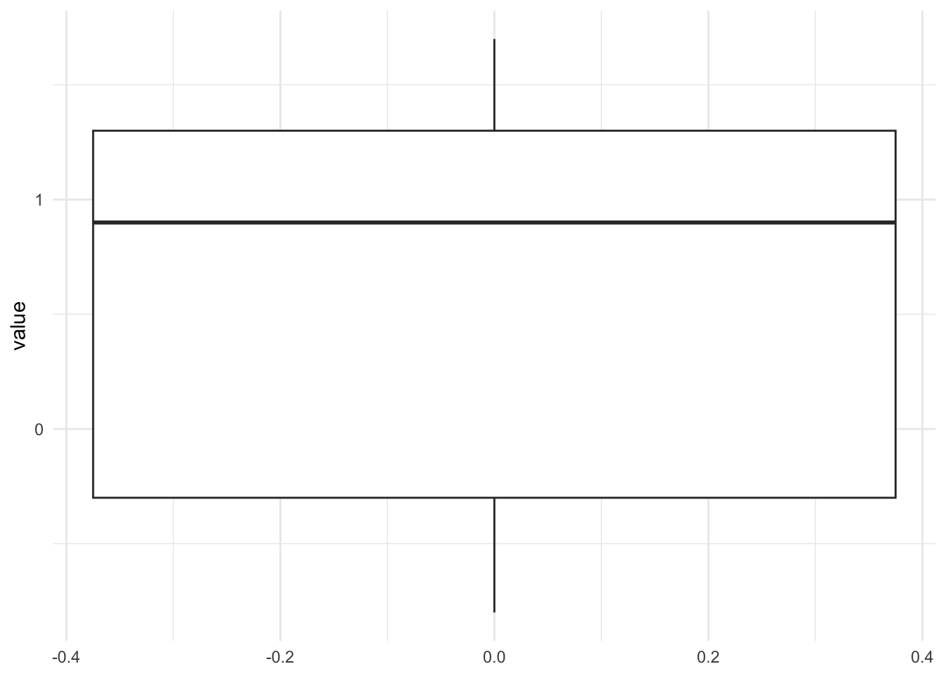
Note that you can use the {esquisse} RStudio addin if you want to draw a boxplot with the package {ggplot2} without writing the code yourself. If you prefer the default graphics, use the boxplot() function:
boxplot(dat1$value)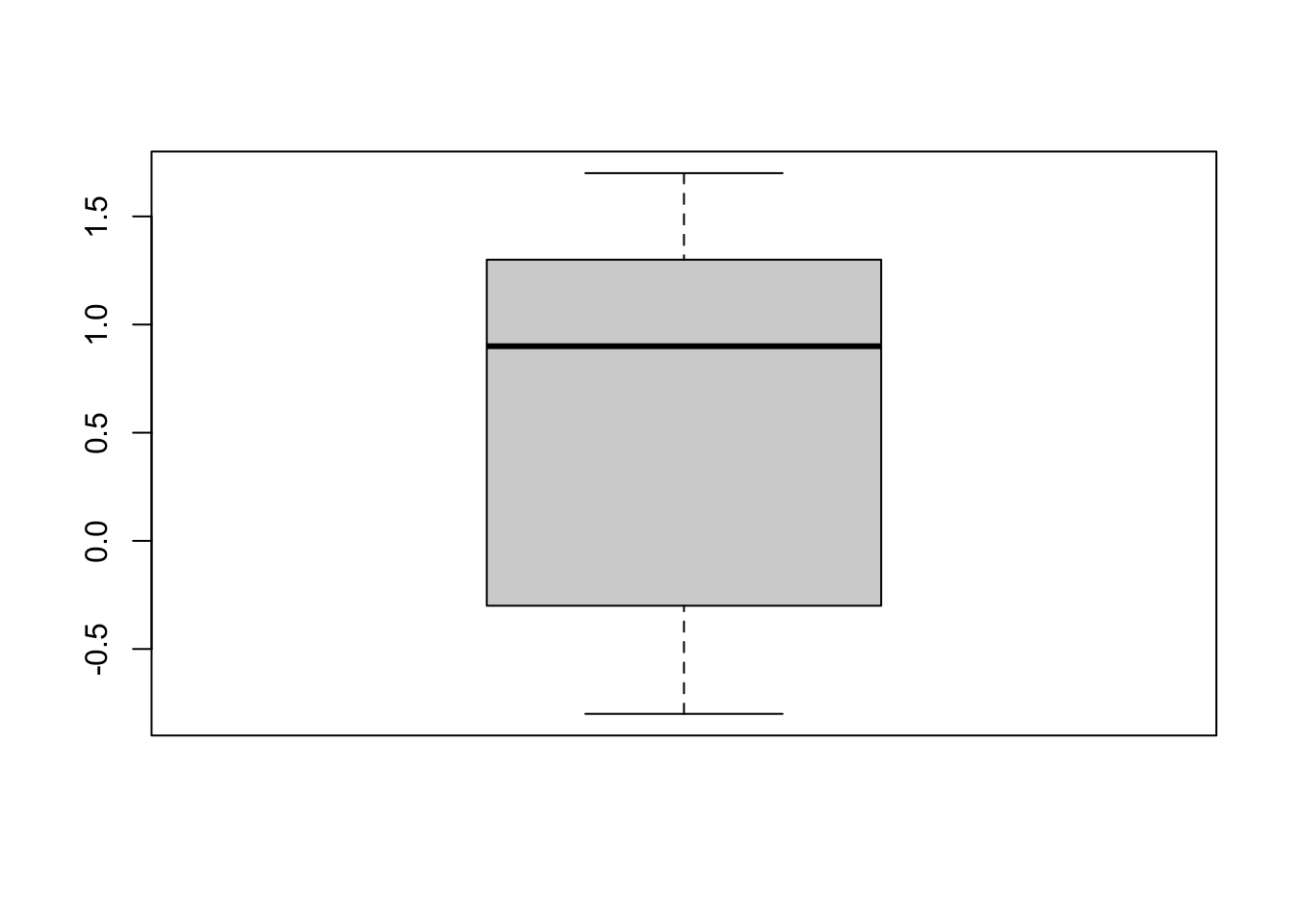
The boxplot shows that the distribution of the sample is not distant from 0 (the hypothesized value), so we tend to believe that we will not be able to reject the null hypothesis that the population mean is equal to 0. However, only a formal statistical test will confirm this belief.
Below a function to perform a t-test with a known population variance, with arguments accepting the sample (x), the variance of the population (V), the mean under the null hypothesis (m0, default is 0), the significance level (alpha, default is 0.05) and the alternative (alternative, one of "two.sided" (default), "less" or "greater"):
t.test2 <- function(x, V, m0 = 0, alpha = 0.05, alternative = "two.sided") {
  M <- mean(x)
  n <- length(x)
  sigma <- sqrt(V)
  S <- sqrt(V / n)
  statistic <- (M - m0) / S
  p <- if (alternative == "two.sided") {
    2 * pnorm(abs(statistic), lower.tail = FALSE)
  } else if (alternative == "less") {
    pnorm(statistic, lower.tail = TRUE)
  } else {
    pnorm(statistic, lower.tail = FALSE)
  }
  LCL <- (M - S * qnorm(1 - alpha / 2))
  UCL <- (M + S * qnorm(1 - alpha / 2))
  value <- list(mean = M, m0 = m0, sigma = sigma, statistic = statistic, p.value = p, LCL = LCL, UCL = UCL, alternative = alternative)
  # print(sprintf("P-value = %g",p))
  # print(sprintf("Lower %.2f%% Confidence Limit = %g",
  #               alpha, LCL))
  # print(sprintf("Upper %.2f%% Confidence Limit = %g",
  #               alpha, UCL))
  return(value)
}

test <- t.test2(dat1$value,
  V = 1
)
test
## $mean
## [1] 0.56
##
## $m0
## [1] 0
##
## $sigma
## [1] 1
##
## $statistic
## [1] 1.252198
##
## $p.value
## [1] 0.2104977
##
## $LCL
## [1] -0.3165225
##
## $UCL
## [1] 1.436523
##
## $alternative
## [1] "two.sided"The output above recaps all the information needed to perform the test: the test statistic, the p-value, the alternative used, the sample mean, the hypothesized value and the population variance (compare these results found in R with the results found by hand).
The p-value can be extracted as usual:
test$p.value## [1] 0.2104977The p-value is 0.21 so at the 5% significance level we do not reject the null hypothesis. There is no sufficient evidence in the data to reject the hypothesis that the population mean is equal to 0. This result confirms what we found by hand.
Note that a similar function exists in the {BSDA} package:2
library(BSDA)

z.test(dat1$value,
  alternative = "two.sided",
  mu = 0,
  sigma.x = 1,
  conf.level = 0.95
)
##
## One-sample z-Test
##
## data: dat1$value
## z = 1.2522, p-value = 0.2105
## alternative hypothesis: true mean is not equal to 0
## 95 percent confidence interval:
## -0.3165225 1.4365225
## sample estimates:
## mean of x
## 0.56If you are unfamiliar with the concept of p-value, I invite you to read my note on p-value and significance level \(\alpha\).
To sum up what have been said in that article about p-value and significance level \(\alpha\):
- If the p-value is smaller than the predetermined significance level \(\alpha\) (usually 5%) so if p-value < 0.05, we reject the null hypothesis
- If the p-value is greater than or equal to the predetermined significance level \(\alpha\) (usually 5%) so if p-value \(\ge\) 0.05, we do not reject the null hypothesis
This applies to all statistical tests without exception. Of course, the null and alternative hypotheses change depending on the test.
Scenario 2: variance of the population is unknown
For the second scenario, suppose the data below. Moreover, suppose that the variance in the population is unknown and that we would like to test whether the population mean is larger than 5.
dat2 <- data.frame(
  value = c(7.9, 5.8, 6.3, 7.3, 6.7)
)

dat2
## value
## 1 7.9
## 2 5.8
## 3 6.3
## 4 7.3
## 5 6.7ggplot(dat2) +
aes(y = value) +
geom_boxplot() +
theme_minimal()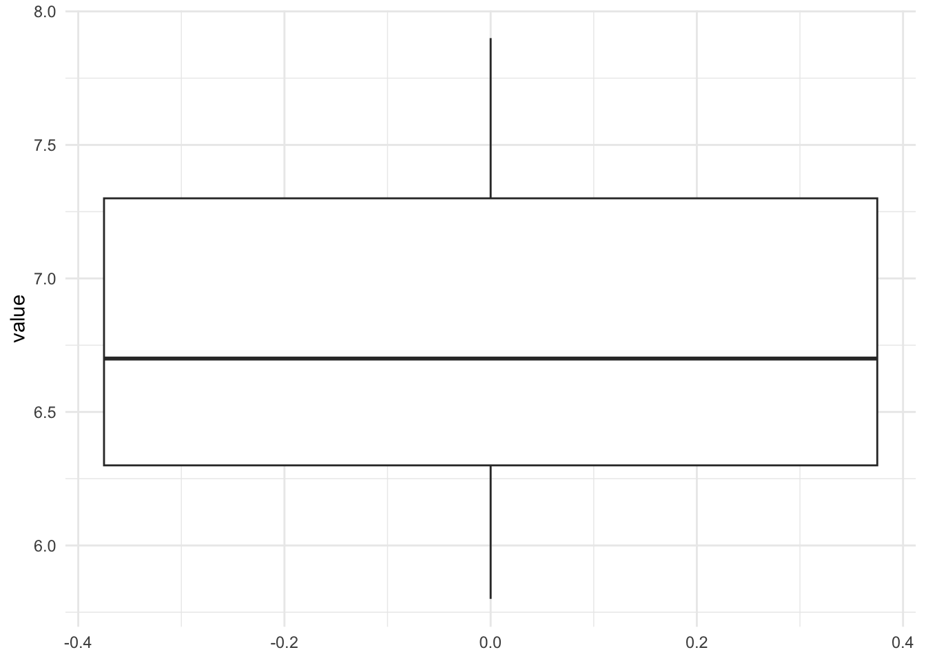
Unlike the previous scenario, the box is quite distant from the hypothesized value of 5. From this boxplot, we can expect the test to reject the null hypothesis of the population mean being equal to 5. Nonetheless, only a formal statistical test will confirm this expectation.
There is a function in R, and it is simply the t.test() function. This version of the test is actually the “standard” t-test for one-sample. Note that in our case the alternative hypothesis is \(H_1: \mu > 5\) so we need to add the arguments mu = 5 and alternative = "greater" to the function because the default arguments are mu = 0 and the two-sided test:
test <- t.test(dat2$value,
  mu = 5,
  alternative = "greater"
)

test
##
## One Sample t-test
##
## data: dat2$value
## t = 4.8809, df = 4, p-value = 0.004078
## alternative hypothesis: true mean is greater than 5
## 95 percent confidence interval:
## 6.013814 Inf
## sample estimates:
## mean of x
## 6.8The output above recaps all the information needed to perform the test: the name of the test, the test statistic, the degrees of freedom, the p-value, the alternative used, the hypothesized value and the sample mean (compare these results found in R with the results found by hand).
The p-value can be extracted as usual:
test$p.value## [1] 0.004077555The p-value is 0.004 so at the 5% significance level we reject the null hypothesis.
Unlike the first scenario, the p-value in this scenario is below 5% so we reject the null hypothesis. At the 5% significance level, we can conclude that the population mean is significantly larger than 5. This result confirms what we found by hand.
Confidence interval
Note that the confidence interval can be extracted with $conf.int:
test$conf.int## [1] 6.013814 Inf
## attr(,"conf.level")
## [1] 0.95You can see that the 95% confidence interval for the population mean is \([6.01; \infty]\), meaning that, at the significance level \(\alpha = 5\)%, we reject the null hypothesis as long as the hypothesized value \(\mu_0\) is below 6.01, otherwise the null hypothesis cannot be rejected.
Combination of plot and statistical test
After having written this article, I discovered the {ggstatsplot} package which I believe is worth mentioning here, in particular the gghistostats() function for one-sample Student’s t-test.
This function combines a histogram—representing the distribution—and the results of the statistical test displayed in the subtitle of the plot.
See examples below for scenario 2. Unfortunately, the package does not allow to run the test for scenario 1.
Scenario 2: variance of the population is unknown
# load packages
library(ggstatsplot)
library(ggplot2)

# plot with stat test
gghistostats(
  data = dat2, # dataframe from which variable is to be taken
  x = value, # numeric variable whose distribution is of interest
  type = "parametric", # for student's t-test
  test.value = 5 # default value is 0
) +
  labs(caption = NULL) # remove caption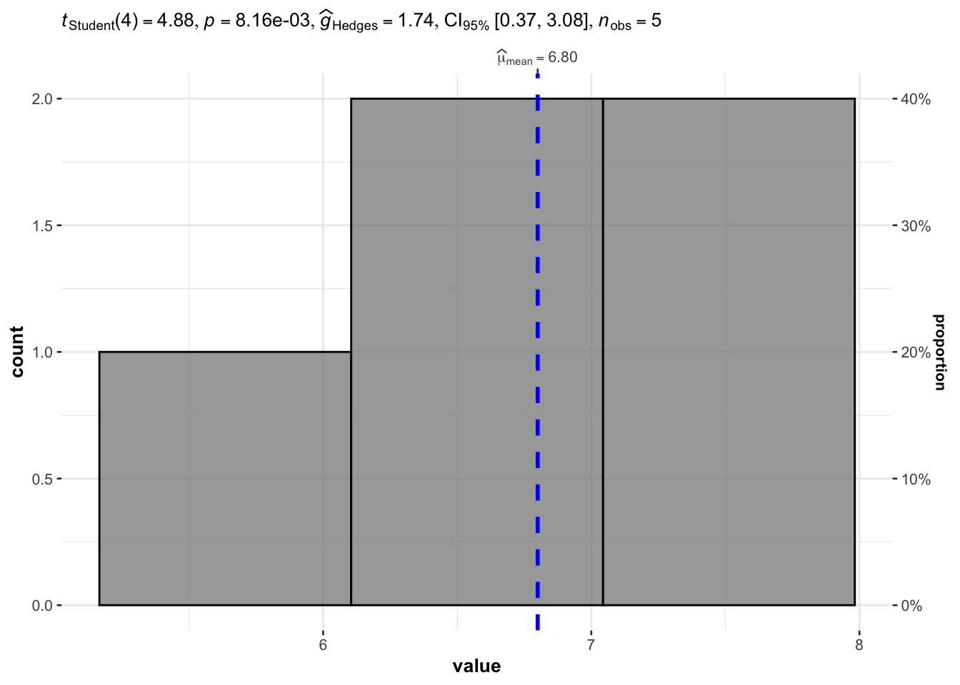
The p-value is displayed after p = in the subtitle of the plot. Based on this plot and the p-value being lower than 5% (p-value = 0.008), we reject the null hypothesis that the population mean is equal to 5.
Note that, the p-value is two times as large as the one obtained with the t.test() function because when we ran t.test() we specified alternative = "greater" (i.e., a one-sided test). In our plot with the gghistostats() function, it is a two-sided test that is performed by default, that is, alternative = "two.sided".
The point of this section was to illustrate how to easily draw plots together with statistical results, which is exactly the aim of the {ggstatsplot} package. See more details and examples in this article.
Assumptions
As for many statistical tests, there are some assumptions that need to be met in order to be able to interpret the results. When one or several assumptions are not met, although it is technically possible to perform these tests, it would be incorrect to interpret the results. Below are the assumptions of the one-sample t-test and how to test them:
- Variable type: The dependent variable (i.e., the measured variable) must be measured on a continuous or ordinal scale.
- Independence: The data, collected from a representative and randomly selected portion of the population, should be independent of one another. The assumption of independence is most often verified based on the design of the experiment and on the good control of experimental conditions rather than via a formal test. If you are still unsure about independence based on the experiment design, ask yourself if one observation is related to another (if one observation has an impact on another). If not, it is most likely that you have independent samples.
- Normality:
- With a small sample size (usually \(n < 30\)), observations should follow a normal distribution. The normality assumption can be tested visually thanks to a histogram and a QQ-plot, and/or formally via a normality test such as the Shapiro-Wilk or Kolmogorov-Smirnov test. Some transformations, such as among others, the logarithm, the square root or the Box-Cox transformation can be applied on the observations to transform you data to better fit the normal distribution. If, even after a transformation, your data still do not follow a normal distribution, the one-sample Wilcoxon test (
wilcox.test(variable_name, data = datin R) can be applied. This non-parametric test is robust to non normal distributions so it does not require normality of the data. - With a large sample size (\(n \ge 30\)), normality of the data is not required (this is a common misconception!). By the central limit theorem, sample means of large samples are often well-approximated by a normal distribution even if the data are not normally distributed (Stevens 2013). It is therefore not required to test the normality assumption when the number of observations is large.
- With a small sample size (usually \(n < 30\)), observations should follow a normal distribution. The normality assumption can be tested visually thanks to a histogram and a QQ-plot, and/or formally via a normality test such as the Shapiro-Wilk or Kolmogorov-Smirnov test. Some transformations, such as among others, the logarithm, the square root or the Box-Cox transformation can be applied on the observations to transform you data to better fit the normal distribution. If, even after a transformation, your data still do not follow a normal distribution, the one-sample Wilcoxon test (
- Outliers: There should be no outliers in your data. An observation slightly different from the others does not pose a problem, but it starts to be an issue when you have at least one extreme outlier. In presence of at least one extreme outlier, it is best to transform your data (with the logarithm transformation for instance, as you would do with a non normal distribution) or use the non-parametric one-sample Wilcoxon test.
Conclusion
Thanks for reading.
I hope this article helped you to understand how the different versions of the one-sample t-test work and how to perform them by hand and in R.
If you are interested, here is a Shiny app to perform these tests by hand easily (you just need to enter your data and select the appropriate version of the test thanks to the sidebar menu). Moreover, read this article if you would like to know how to compute the Student’s t-test but this time, for two samples—in order to compare two dependent or independent groups—or this article if you want to use an ANOVA to compare 3 or more groups.
As always, if you have a question or a suggestion related to the topic covered in this article, please add it as a comment so other readers can benefit from the discussion.
References
It is a least the case regarding parametric hypothesis tests. A parametric test means that it is based on a theoretical statistical distribution, which depends on some defined parameters. In the case of the one-sample t-test, it is based on the Student’s t distribution with a single parameter, the degrees of freedom (\(df = n - 1\) where \(n\) is the sample size), or the normal distribution.↩︎
Thanks gmacar for pointing it out to me.↩︎
Liked this post?
- Get updates every time a new article is published (no spam and unsubscribe anytime)
- Support the blog
- Share on:


