
Outliers detection in R

Introduction
An outlier is a value or an observation that is distant from other observations, that is to say, a data point that differs significantly from other data points. Enderlein (1987) goes even further as the author considers outliers as values that deviate so much from other observations one might suppose a different underlying sampling mechanism.
An observation must always be compared to other observations made on the same phenomenon before actually calling it an outlier. Indeed, someone who is 200 cm tall (6’7” in US) will most likely be considered as an outlier compared to the general population, but that same person may not be considered as an outlier if we measured the height of basketball players.
An outlier may be due to the variability inherent in the observed phenomenon. For example, it is often the case that there are outliers when collecting data on salaries, as some people make much more money than the rest.
Outliers can also arise due to an experimental, measurement or encoding error. For instance, a human weighting 786 kg (1733 pounds) is clearly an error when encoding the weight of the subject. Her or his weight is most probably 78.6 kg (173 pounds) or 7.86 kg (17 pounds) depending on whether weights of adults or babies have been measured.
For this reason, it sometimes makes sense to formally distinguish two classes of outliers: (i) extreme values and (ii) mistakes. Extreme values are statistically and philosophically more interesting, because they are possible but unlikely responses.1
In this article, I present several approaches to detect outliers in R, from simple techniques such as descriptive statistics (including minimum, maximum, histogram, boxplot and percentiles) to more formal techniques such as the Hampel filter, the Grubbs, the Dixon and the Rosner tests for outliers.
Although there is no strict or unique rule whether outliers should be removed or not from the dataset before doing statistical analyses, it is quite common to, at least, remove or impute outliers that are due to an experimental or measurement error (like the weight of 786 kg (1733 pounds) for a human). Some statistical tests require the absence of outliers in order to draw sound conclusions, but removing outliers is not recommended in all cases and must be done with caution.
This article will not tell you whether you should remove outliers or not (nor if you should impute them with the median, mean, mode or any other value), but it will help you to detect them in order to, as a first step, verify them. After their verification, it is then your choice to exclude or include them for your analyses (and this usually requires a thoughtful reflection on the researcher’s side).
Removing or keeping outliers mostly depend on three factors:
- The domain/context of your analyses and the research question. In some domains, it is common to remove outliers as they often occur due to a malfunctioning process. In other fields, outliers are kept because they contain valuable information. It also happens that analyses are performed twice, once with and once without outliers to evaluate their impact on the conclusions. If results change drastically due to some influential values, this should caution the researcher to make overambitious claims.
- Whether the tests you are going to apply are robust to the presence of outliers or not. For instance, the slope of a simple linear regression may significantly varies with just one outlier, whereas non-parametric tests such as the Wilcoxon test are usually robust to outliers.
- How distant are the outliers from other observations? Some observations considered as outliers (according to the techniques presented below) are actually not really extreme compared to all other observations, while other potential outliers may be really distant from the rest of the observations.
The dataset mpg from the {ggplot2} package will be used to illustrate the different approaches of outliers detection in R, and in particular we will focus on the variable hwy (highway miles per gallon). We will also use some simulated data for the presentation of the outlier tests.
Descriptive statistics
Several methods using descriptive statistics exist. We present the most common ones below.
Minimum and maximum
The first step to detect outliers in R is to start with some descriptive statistics, and in particular with the minimum and maximum.
In R, this can easily be done with the summary() function:
dat <- ggplot2::mpg
summary(dat$hwy)
## Min. 1st Qu. Median Mean 3rd Qu. Max.
## 12.00 18.00 24.00 23.44 27.00 44.00where the minimum and maximum are respectively the first and last values in the output above.
Alternatively, they can also be computed with the min() and max(), or range() functions:2
min(dat$hwy)## [1] 12max(dat$hwy)## [1] 44range(dat$hwy)## [1] 12 44Some clear encoding mistake like a weight of 786 kg (1733 pounds) for a human will already be easily detected by this very simple technique.
Histogram
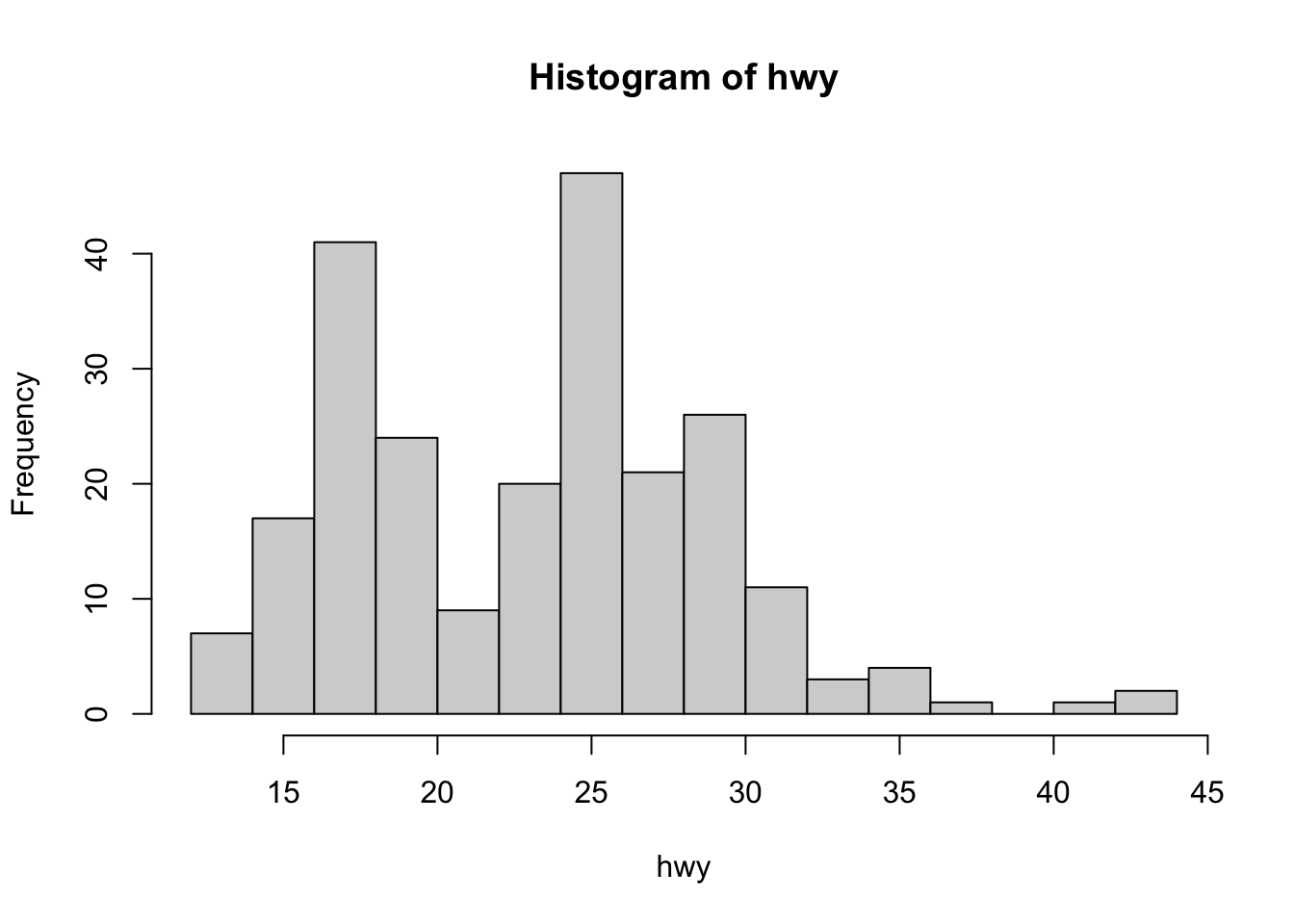
Another basic way to detect outliers is to draw a histogram of the data.
Using R base (with the number of bins corresponding to the square root of the number of observations in order to have more bins than the default option):
hist(dat$hwy,
  xlab = "hwy",
  main = "Histogram of hwy",
  breaks = sqrt(length(dat$hwy)) # set number of bins
)
or using ggplot2 (learn how to create plots with this package via the esquisse addin or via this tutorial):
library(ggplot2)

ggplot(dat) +
  aes(x = hwy) +
  geom_histogram(
    bins = round(sqrt(length(dat$hwy))), # set number of bins
    fill = "steelblue", color = "black"
  ) +
  theme_minimal()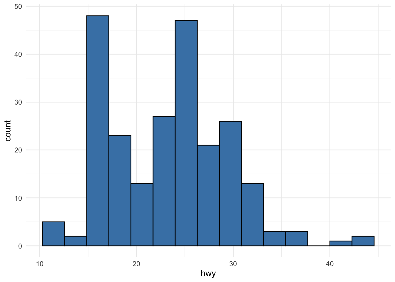
From the histograms, we see that there seems to be a couple of observations larger than all other observations (see the bars on the right side of the plot).
Boxplot
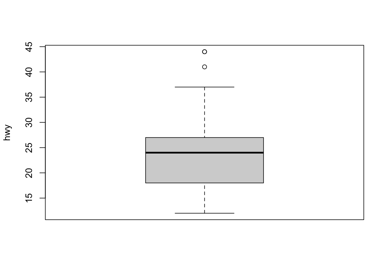
In addition to histograms, boxplots are also useful to detect potential outliers.
Using R base:
boxplot(dat$hwy,
  ylab = "hwy"
)
or using ggplot2:
ggplot(dat) +
  aes(x = "", y = hwy) +
  geom_boxplot(fill = "steelblue") +
  theme_minimal()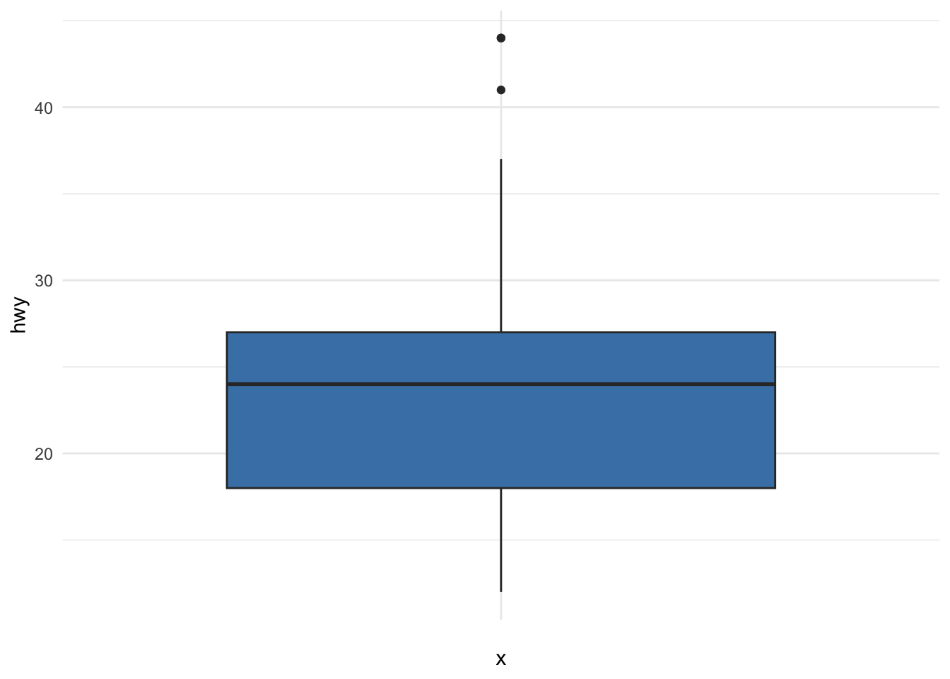
A boxplot helps to visualize a quantitative variable by displaying five common location summary (minimum, median, first and third quartiles and maximum) and any observation that was classified as a suspected outlier using the interquartile range (IQR) criterion.
The IQR criterion means that all observations above \(q_{0.75} + 1.5 \cdot IQR\) or below \(q_{0.25} - 1.5 \cdot IQR\) (where \(q_{0.25}\) and \(q_{0.75}\) correspond to first and third quartile respectively, and IQR is the difference between the third and first quartile) are considered as potential outliers by R.
In other words, all observations outside of the following interval will be considered as potential outliers:
\[I = [q_{0.25} - 1.5 \cdot IQR; q_{0.75} + 1.5 \cdot IQR]\]
Observations considered as potential outliers by the IQR criterion are displayed as points in the boxplot. Based on this criterion, there are 2 potential outliers (see the 2 points above the vertical line, at the top of the boxplot).
Remember that it is not because an observation is considered as a potential outlier by the IQR criterion that you should remove it. Removing or keeping an outlier depends on:
- the context of your analysis,
- whether the tests you are going to perform on the dataset are robust to outliers or not, and
- how extreme is the outlier (so how far is the outlier from other observations).
It is also possible to extract the values of the potential outliers based on the IQR criterion thanks to the boxplot.stats()$out function:
boxplot.stats(dat$hwy)$out## [1] 44 44 41As you can see, there are actually 3 points considered as potential outliers: 2 observations with a value of 44 and 1 observation with a value of 41.
Thanks to the which() function it is possible to extract the row number corresponding to these outliers:
out <- boxplot.stats(dat$hwy)$out
out_ind <- which(dat$hwy %in% c(out))
out_ind
## [1] 213 222 223With this information you can now easily go back to the specific rows in the dataset to verify them, or print all variables for these outliers:
dat[out_ind, ]## # A tibble: 3 × 11
## manufacturer model displ year cyl trans drv cty hwy fl class
## <chr> <chr> <dbl> <int> <int> <chr> <chr> <int> <int> <chr> <chr>
## 1 volkswagen jetta 1.9 1999 4 manua… f 33 44 d comp…
## 2 volkswagen new beetle 1.9 1999 4 manua… f 35 44 d subc…
## 3 volkswagen new beetle 1.9 1999 4 auto(… f 29 41 d subc…Another method to display these specific rows is with the identify_outliers() function from the {rstatix} package:3
library(rstatix)

identify_outliers(
  data = dat,
  variable = "hwy"
)
## # A tibble: 3 × 13
## manufacturer model displ year cyl trans drv cty hwy fl class
## <chr> <chr> <dbl> <int> <int> <chr> <chr> <int> <int> <chr> <chr>
## 1 volkswagen jetta 1.9 1999 4 manua… f 33 44 d comp…
## 2 volkswagen new beetle 1.9 1999 4 manua… f 35 44 d subc…
## 3 volkswagen new beetle 1.9 1999 4 auto(… f 29 41 d subc…
## # ℹ 2 more variables: is.outlier <lgl>, is.extreme <lgl>It is also possible to print the values of the outliers directly on the boxplot with the mtext() function:
boxplot(dat$hwy,
  ylab = "hwy",
  main = "Boxplot of highway miles per gallon"
)
mtext(paste("Outliers: ", paste(out, collapse = ", ")))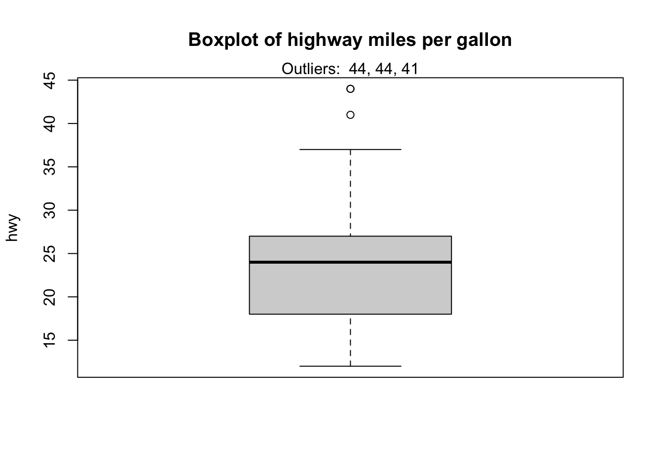
Percentiles
This method of outliers detection is based on the percentiles.
With the percentiles method, all observations that lie outside the interval formed by the 2.5 and 97.5 percentiles will be considered as potential outliers. Other percentiles such as the 1 and 99, or the 5 and 95 percentiles can also be considered to construct the interval.
The values of the lower and upper percentiles (and thus the lower and upper limits of the interval) can be computed with the quantile() function:
lower_bound <- quantile(dat$hwy, 0.025)
lower_bound
## 2.5%
## 14upper_bound <- quantile(dat$hwy, 0.975)
upper_bound## 97.5%
## 35.175According to this method, all observations below 14 and above 35.175 will be considered as potential outliers. The row numbers of the observations outside of the interval can then be extracted with the which() function:
outlier_ind <- which(dat$hwy < lower_bound | dat$hwy > upper_bound)
outlier_ind
## [1] 55 60 66 70 106 107 127 197 213 222 223Then their values of highway miles per gallon can be printed:
dat[outlier_ind, "hwy"]## # A tibble: 11 × 1
## hwy
## <int>
## 1 12
## 2 12
## 3 12
## 4 12
## 5 36
## 6 36
## 7 12
## 8 37
## 9 44
## 10 44
## 11 41Alternatively, all variables for these outliers can be printed:
dat[outlier_ind, ]## # A tibble: 11 × 11
## manufacturer model displ year cyl trans drv cty hwy fl class
## <chr> <chr> <dbl> <int> <int> <chr> <chr> <int> <int> <chr> <chr>
## 1 dodge dakota pi… 4.7 2008 8 auto… 4 9 12 e pick…
## 2 dodge durango 4… 4.7 2008 8 auto… 4 9 12 e suv
## 3 dodge ram 1500 … 4.7 2008 8 auto… 4 9 12 e pick…
## 4 dodge ram 1500 … 4.7 2008 8 manu… 4 9 12 e pick…
## 5 honda civic 1.8 2008 4 auto… f 25 36 r subc…
## 6 honda civic 1.8 2008 4 auto… f 24 36 c subc…
## 7 jeep grand che… 4.7 2008 8 auto… 4 9 12 e suv
## 8 toyota corolla 1.8 2008 4 manu… f 28 37 r comp…
## 9 volkswagen jetta 1.9 1999 4 manu… f 33 44 d comp…
## 10 volkswagen new beetle 1.9 1999 4 manu… f 35 44 d subc…
## 11 volkswagen new beetle 1.9 1999 4 auto… f 29 41 d subc…There are 11 potential outliers according to the percentiles method. To reduce this number, you can set the percentiles to 1 and 99:
lower_bound <- quantile(dat$hwy, 0.01)
upper_bound <- quantile(dat$hwy, 0.99)

outlier_ind <- which(dat$hwy < lower_bound | dat$hwy > upper_bound)

dat[outlier_ind, ]
## # A tibble: 3 × 11
## manufacturer model displ year cyl trans drv cty hwy fl class
## <chr> <chr> <dbl> <int> <int> <chr> <chr> <int> <int> <chr> <chr>
## 1 volkswagen jetta 1.9 1999 4 manua… f 33 44 d comp…
## 2 volkswagen new beetle 1.9 1999 4 manua… f 35 44 d subc…
## 3 volkswagen new beetle 1.9 1999 4 auto(… f 29 41 d subc…Setting the percentiles to 1 and 99 gives the same potential outliers as with the IQR criterion.
Z-scores
If your data come from a normal distribution, you can use the z-scores, defined as
\[z_i = \frac{x_i - \overline{X}}{s_X}\]
where \(\overline{X}\) is the mean and \(s_X\) is the standard deviation of the random variable \(X\).
This is referred as scaling, which can be done with the scale() function in R.
According to this method, any z-score:
- < -2 or > 2 is considered as rare
- < -3 or > 3 is considered as extremely rare
Other authors also use a z-score below -3.29 or above 3.29 to detect outliers. This value of 3.29 comes from the fact that 1 observation out of 1000 is out of this interval if the data follow a normal distribution.
In our case:
dat$z_hwy <- scale(dat$hwy)

hist(dat$z_hwy)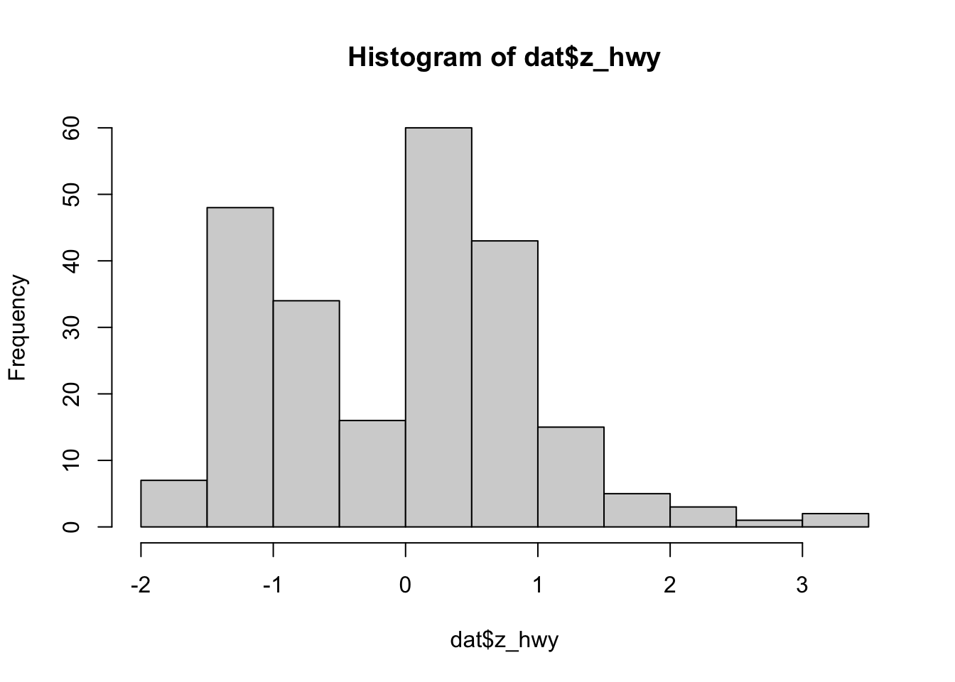
summary(dat$z_hwy)## V1
## Min. :-1.92122
## 1st Qu.:-0.91360
## Median : 0.09402
## Mean : 0.00000
## 3rd Qu.: 0.59782
## Max. : 3.45274We see that there are some observations above 3.29, but none below -3.29.
To identify the line in the dataset of these observations:
which(dat$z_hwy > 3.29)## [1] 213 222We see that observations 213 and 222 can be considered as outliers according to this method.
Hampel filter
Another method, known as Hampel filter, consists of considering as outliers the values outside the interval (\(I\)) formed by the median, plus or minus 3 median absolute deviations (\(MAD\)):4
\[I = [median - 3 \cdot MAD; median + 3 \cdot MAD]\]
where \(MAD\) is the median absolute deviation and is defined as the median of the absolute deviations from the data’s median \(\tilde{X} = median(X)\):
\[MAD = median(|X_i - \tilde{X}|)\]
For this method we first set the interval limits thanks to the median() and mad() functions:5
lower_bound <- median(dat$hwy) - 3 * mad(dat$hwy, constant = 1)
lower_bound
## [1] 9upper_bound <- median(dat$hwy) + 3 * mad(dat$hwy, constant = 1)
upper_bound## [1] 39According to this method, all observations below 9 and above 39 will be considered as potential outliers. The row numbers of the observations outside of the interval can then be extracted with the which() function:
outlier_ind <- which(dat$hwy < lower_bound | dat$hwy > upper_bound)
outlier_ind
## [1] 213 222 223According to the Hampel filter, there are 3 outliers for the hwy variable.
Statistical tests
In this section, we present 3 hypothesis tests to detect outliers:
- Grubbs’s test
- Dixon’s test
- Rosner’s test
These 3 statistical tests are part of more formal techniques of outliers detection as they all involve the computation of a test statistic that is compared to tabulated critical values (that are based on the sample size and the desired confidence level).
Note that the 3 tests are appropriate only when the data, without any outliers, are approximately normally distributed. It is recommended to check normality visually, with a QQ-plot, a histogram and/or a boxplot for instance. Although it can also be checked with a formal test for normality (such as the Shapiro-Wilk test for example), the presence of one or more outliers may cause the normality test to reject normality when it is in fact a reasonable assumption for applying one of the 3 outlier tests mentioned above.
We check the normality of our data thanks to a QQ-plot:
library(car)
qqPlot(dat$hwy)
## [1] 213 222Too many points deviate from the Henry’s line, so based on the QQ-plot we conclude that our data do not follow a normal distribution. Therefore, we should not use one of the outlier test on these data.
For the sake of completeness, here is an example of data that could be used with the three outlier tests, together with the QQ-plot of these data:
dat_tests <- c(rnorm(50), 5)

qqPlot(dat_tests)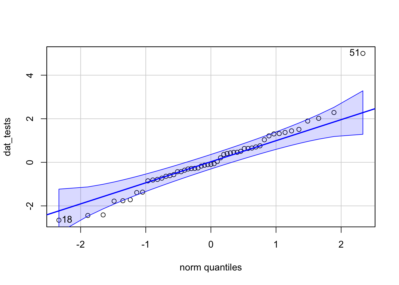
## [1] 51 18hist(dat_tests)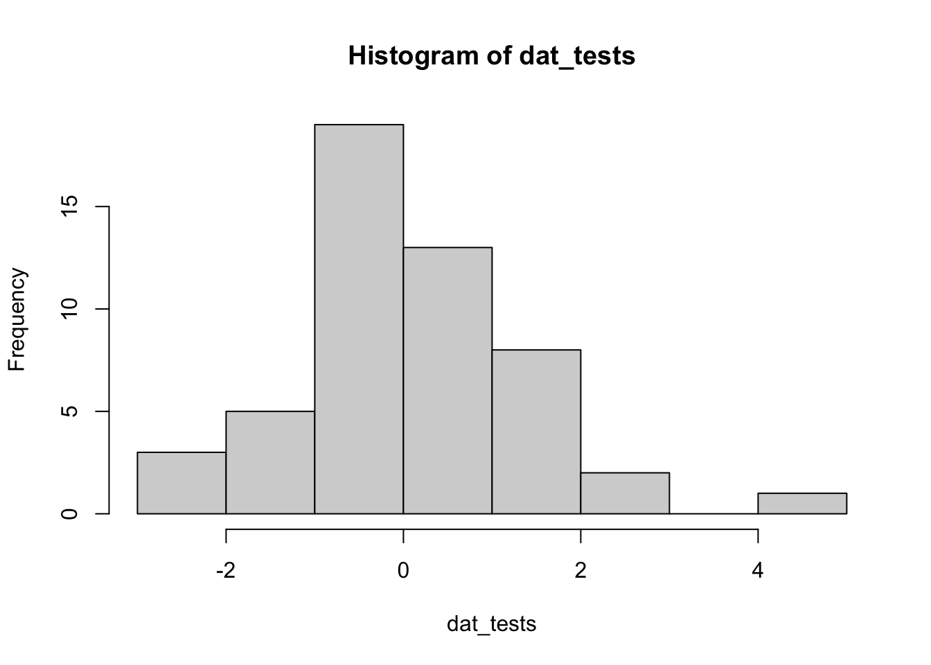
For the illustration of the three outlier tests in the next sections, we thus use the simulated data (dat_tests) instead of the data used so far (dat$hwy).
Grubbs’s test
The Grubbs test allows to detect whether the highest or lowest value in a dataset is an outlier.
The Grubbs test detects one outlier at a time (highest or lowest value), so the null and alternative hypotheses are as follows:
- \(H_0\): The highest value is not an outlier
- \(H_1\): The highest value is an outlier
if we want to test the highest value, or:
- \(H_0\): The lowest value is not an outlier
- \(H_1\): The lowest value is an outlier
if we want to test the lowest value.
As for any statistical test, if the p-value is less than the chosen significance threshold (generally \(\alpha = 0.05\)) then the null hypothesis is rejected and we will conclude that the lowest/highest value is an outlier.
On the contrary, if the p-value is greater or equal than the significance level, the null hypothesis is not rejected, and we will conclude that, based on the data, we do not reject the hypothesis that the lowest/highest value is not an outlier.
Note that the Grubbs test is not appropriate for sample size of 6 or less (\(n \le 6\)).
To perform the Grubbs test in R, we use the grubbs.test() function from the {outliers} package:
# install.packages("outliers")
library(outliers)

# Grubbs test
test <- grubbs.test(dat_tests)
test
##
## Grubbs test for one outlier
##
## data: dat_tests
## G = 3.68326, U = 0.72325, p-value = 0.001873
## alternative hypothesis: highest value 5 is an outlierThe p-value is 0.002. At the 5% significance level, we reject the hypothesis that the highest value 5 is not an outlier. In other words, based on this test, we conclude that the highest value 5 is an outlier.
By default, the test is performed on the highest value (as shown in the R output: alternative hypothesis: highest value 5 is an outlier). If you want to do the test for the lowest value, simply add the argument opposite = TRUE in the grubbs.test() function:
test <- grubbs.test(dat_tests, opposite = TRUE)
test
##
## Grubbs test for one outlier
##
## data: dat_tests
## G = 2.02893, U = 0.91602, p-value = 0.9981
## alternative hypothesis: lowest value -2.65645542090478 is an outlierThe R output indicates that the test is now performed on the lowest value (see alternative hypothesis: lowest value -2.6564554 is an outlier).
The p-value is 0.998. At the 5% significance level, we do not reject the hypothesis that the lowest value -2.66 is not an outlier. In other words, we cannot conlude that the lowest value -2.66 is an outlier.
Dixon’s test
Similar to the Grubbs test, Dixon test is used to test whether a single low or high value is an outlier. So if more than one outliers is suspected, the test has to be performed on these suspected outliers individually.
Note that Dixon test is most useful for small sample size (usually \(n \le 25\)).
To perform the Dixon’s test in R, we use the dixon.test() function from the {outliers} package.
For this illustration, as the Dixon test can only be done on small samples, we take a subset of our simulated data which consists of the 20 first observations and the outlier. Note that R will throw an error and accepts only a dataset consisting of 3 to 30 observations for this test.
# subset of simulated data
subdat <- c(dat_tests[1:20], max(dat_tests))

# Dixon test
test <- dixon.test(subdat)
test
##
## Dixon test for outliers
##
## data: subdat
## Q = 0.46668, p-value = 0.06429
## alternative hypothesis: highest value 5 is an outlierResults of the Dixon test show that we cannot conclude that the highest value 5 is an outlier (p-value = 0.064).
To test for the lowest value, simply add the opposite = TRUE argument to the dixon.test() function:
test <- dixon.test(subdat,
  opposite = TRUE
)
test
##
## Dixon test for outliers
##
## data: subdat
## Q = 0.27115, p-value = 0.6872
## alternative hypothesis: lowest value -2.65645542090478 is an outlierResults of the test show that we cannot conclude that the lowest value -2.66 is an outlier (p-value = 0.687).
It is a good practice to always check the results of the statistical test for outliers against the boxplot to make sure we tested all potential outliers:
out <- boxplot.stats(subdat)$out

boxplot(subdat)
mtext(paste("Outlier: ", paste(out, collapse = ", ")))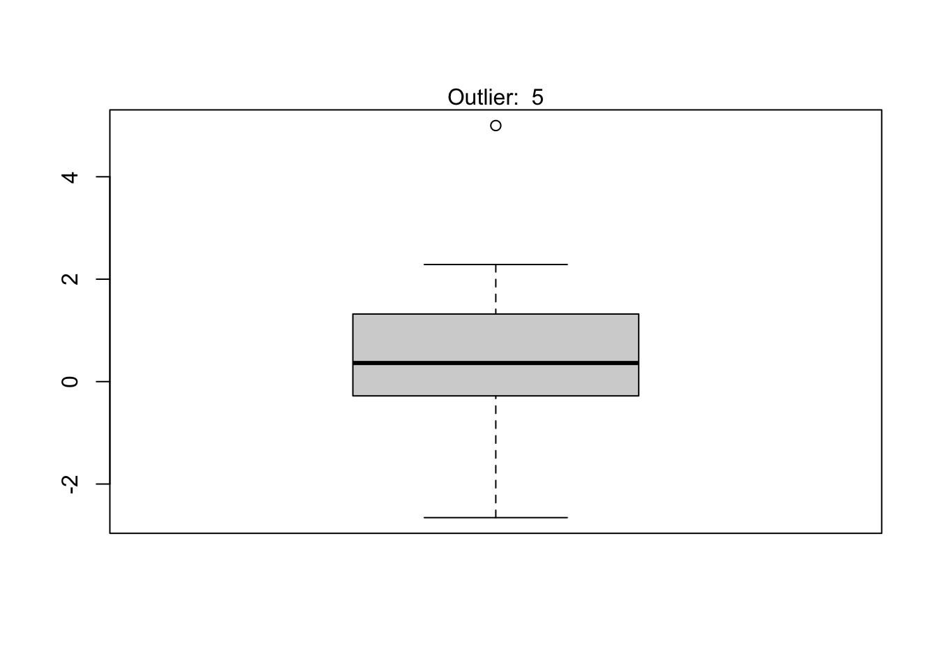
From the boxplot, we see that the Dixon test has been applied to all potential outliers.
If you need to perform the test again without the highest or lowest value, this can be done by finding the row number of the maximum or minimum value, excluding this row number from the dataset and then finally apply the Dixon test on this new dataset. We illustrate the process as if we needed to perform the test again, but this time on the data excluding the highest value:
# find and exclude highest value
remove_ind <- which.max(subdat)
subsubdat <- subdat[-remove_ind]

# Dixon test on dataset without the maximum
test <- dixon.test(subsubdat)
test
##
## Dixon test for outliers
##
## data: subsubdat
## Q = 0.30413, p-value = 0.5547
## alternative hypothesis: lowest value -2.65645542090478 is an outlierResults show that we cannot conclude that the lowest value -2.66 is an outlier (p-value = 0.555).
Rosner’s test
Rosner’s test for outliers has the advantages that:
- it is used to detect several outliers at once (unlike Grubbs and Dixon test which must be performed iteratively to screen for multiple outliers), and
- it is designed to avoid the problem of masking, where an outlier that is close in value to another outlier can go undetected.
Unlike Dixon test, note that Rosner test is most appropriate when the sample size is large (\(n \ge 20\)). We therefore use again the similated dataset (i.e., dat_tests), which includes 51 observations.
To perform the Rosner test, we use the rosnerTest() function from the {EnvStats} package. This function requires at least 2 arguments: the data and the number of suspected outliers k (with k = 3 as the default number of suspected outliers).
For this example, we set the number of suspected outliers to be equal to 1, as suggested by the number of potential outliers outlined in the boxplot.6
library(EnvStats)

# Rosner test
test <- rosnerTest(dat_tests,
  k = 1
)
test
##
## Results of Outlier Test
## -------------------------
##
## Test Method: Rosner's Test for Outliers
##
## Hypothesized Distribution: Normal
##
## Data: dat_tests
##
## Sample Size: 51
##
## Test Statistic: R.1 = 3.683258
##
## Test Statistic Parameter: k = 1
##
## Alternative Hypothesis: Up to 1 observations are not
## from the same Distribution.
##
## Type I Error: 5%
##
## Number of Outliers Detected: 1
##
##   i     Mean.i     SD.i Value Obs.Num    R.i+1 lambda.i+1 Outlier
## 1 0 0.06306688 1.340371 5 51 3.683258 3.136165 TRUEThe interesting results are provided in the $all.stats table:
test$all.stats## i Mean.i SD.i Value Obs.Num R.i+1 lambda.i+1 Outlier
## 1 0 0.06306688 1.340371 5 51 3.683258 3.136165 TRUEBased on the results of the Rosner test, we see that there is only one outlier (as the table contains 1 line), and that it is the observation 51 (see Obs.Num) with a value of 5 (see Value). This finding aligns with the Grubbs test presented above, which also detected the value 5 as an outlier.
Additional remarks
You will find many other methods to detect outliers:
- in the
{outliers}packages, - via the
lofactor()function from the{DMwR}package: Local Outlier Factor (LOF) is an algorithm used to identify outliers by comparing the local density of a point with that of its neighbors, - the
outlierTest()from the{car}package gives the most extreme observation based on the given model and allows to test whether it is an outlier, - in the
{OutlierDetection}package, and - with the
aq.plot()function from the{mvoutlier}package (Thanks KTR for the suggestion.).
We present these methods with the initial dataset mpg, using the cyl and hwy variables:
library(mvoutlier)

Y <- as.matrix(ggplot2::mpg[, c("cyl", "hwy")])
res <- aq.plot(Y)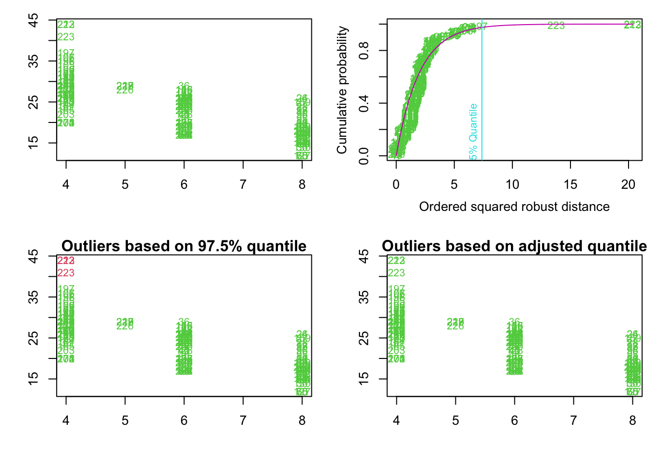
Note also that some transformations may “naturally” eliminate outliers. The natural log or square root of a value reduces the variation caused by extreme values, so in some cases applying these transformations will help in making potential outliers less extreme.
Conclusion
Thanks for reading.
I hope this article helped you to detect outliers in R via several descriptive statistics (including minimum, maximum, histogram, boxplot and percentiles) or thanks to more formal techniques of outliers detection (including Hampel filter, Grubbs, Dixon and Rosner tests).
It is now your turn to try to detect outliers in your data, and decide how to treat them (i.e., keeping, removing or imputing them) before conducting your analyses.
As always, if you have a question or a suggestion related to the topic covered in this article, please add it as a comment so other readers can benefit from the discussion.
(Note that this article is available for download on my Gumroad page.)
References
Thanks Felix Kluxen for the valuable suggestion.↩︎
Thanks to Victor for pointing out the
range()function.↩︎Thanks to Marlenildo for pointing out the
identify_outliers()function.↩︎The default is 3 (according to Pearson’s rule), but another value is also possible.↩︎
The constant in the
mad()function is 1.4826 by default, so it has to be set to 1 to find the median absolute deviation. Seehelp(mad)for more details. Thanks to Elisei for pointing this out to me.↩︎In order to avoid flawed conclusions, it is important to pre-screen the data (graphically with a boxplot for example) to make the selection of the number of potential outliers as accurate as possible prior to running Rosner’s test.↩︎
Liked this post?
- Get updates every time a new article is published (no spam and unsubscribe anytime)
- Support the blog
- Share on:


