
The 9 concepts and formulas in probability that every data scientist should know

What is probability?
A probability is a number that reflects the chance that a particular event will occur. In other words, it quantifies (on a scale from 0 to 1, or from 0% to 100%) how likely an event is to occur.
Probability is a branch of mathematics that provides models to describe random processes. These mathematical tools allow to establish theoretical models for random phenomena and to use them to make predictions. Like every model, the probabilistic model is a simplification of the world. However, the model is useful as soon as it captures the essential features.
In this article, we present 9 fundamental formulas and concepts in probability that every data scientist should understand and master in order to appropriately handle any project involving probabilities.
1. A probability is always between 0 and 1
The probability of an event is always between 0 and 1 (or 0% and 100%). If we denote the probability that an event A (which could be any event) occurs by \(P(A)\), we have:
\[0 \le P(A) \le 1\]
- If an event is impossible: \(P(A) = 0\)
- If an event is certain: \(P(A) = 1\)
For example, throwing a 7 with a standard six-sided dice (with faces ranging from 1 to 6) is impossible so its probability is equal to 0. Throwing head or tail with a coin is certain, so its probability is equal to 1.
2. Compute a probability
If the elements of a sample space (the set of all possible results of a randomized experiment) are equiprobable (= all elements have the same probability), then the probability of an event occurring is equal to the number of favourable cases (number of ways it can happen) divided by the number of possible cases (total number of outcomes):
\[P(A) = \frac{\text{number of favourable cases}}{\text{number of possible cases}}\]
For example, all numbers of a six-sided dice are equiprobable since they all have the same probability of occurring. The probability of rolling a 3 with a dice is thus
\[P(3) = \frac{\text{number of favourable cases}}{\text{number of possible cases}} = \frac{1}{6}\]
because there is only one favourable case (there is only one face with a 3 on it), and there are 6 possible cases (because there are 6 faces altogether).
3. Complement of an event
The probability of the complement (or opposite) of an event is:
\[P(\text{not A}) = P(\bar{A}) = 1 - P(A)\]
For instance, the probability of not throwing a 3 with a dice is:
\[P(\bar{A}) = 1 - P(A) = 1 - \frac{1}{6} = \frac{5}{6}\]
4. Union of two events
The probability of the union of two events is the probability of either occurring:
\[\begin{align} P(\text{A or B)} &= P(A \cup B) \\ &= P(A) + P(B) - P(A \cap B) \end{align}\]
Suppose that the probability of a fire breaking out in two houses in a given year is:
- in house A: 60%, so \(P(A) = 0.6\)
- in house B: 45%, so \(P(B) = 0.45\)
- in at least one of the two houses: 80%, so \(P(A \cup B) = 0.8\)
Graphically we have
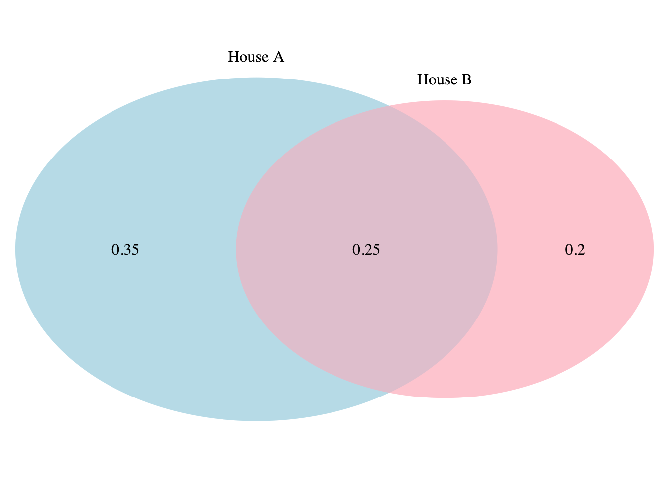
The probability of a fire breaking out in house A or house B is
\[P(A \cup B) = P(A) + P(B) - P(A \cap B)\] \[= 0.6 + 0.45 - 0.25 = 0.8\]
By summing \(P(A)\) and \(P(B)\), the intersection of A and B, i.e. \(P(A \cap B)\), is counted twice. This is the reason we subtract it to count it only once.
If two events are mutually exclusive (i.e., two events that cannot occur simultaneously), the probability of both events occurring \(P(A \cap B)\) is equal to 0, so the above formula becomes
\[P(A \cup B) = P(A) + P(B)\]
For example, the event “rolling a 3” and the event “rolling a 6” on a six-sided dice are two mutually exclusive events since they cannot both occur at the same time. Since their joint probability is equal to 0, the probability of rolling a 3 or 6 on a six-sided dice is
\[P(3 \cup 6) = P(3) + P(6) = \frac{1}{6} + \frac{1}{6} = \frac{1}{3}\]
5. Intersection of two events
If two events are independent, the probability of the intersection of the two events (i.e., the joint probability) is the probability of the two events occurring:
\[P(\text{A and B)} = P(A \cap B) = P(A) \cdot P(B)\]
For instance, if two coins are flipped, the probability of both coins being tails is
\[P(T_1 \cap T_2) = P(T_1) \cdot P(T_2) = \frac{1}{2} \cdot \frac{1}{2} = \frac{1}{4}\]
where \(T_1\) (\(T_2\)) denotes the event that the first (second) coin is tail.
Note that \(P(A \cap B) = P(B \cap A)\).
If two events are mutually exclusive, their joint probability is equal to 0:
\[P(A \cap B) = 0\]
6. Independence of two events
Another important concept in probability is the independence of two events. Formally, the events A and B are independent if and only if
\[P(A \cap B) = P(A) \cdot P(B)\]
If the equality holds, the two events are said to be independent, otherwise the two events are said to be dependent.
- In the example of the two coins:
\[P(T_1 \cap T_2) = \frac{1}{4}\]
and
\[P(T_1) \cdot P(T_2) = \frac{1}{2} \cdot \frac{1}{2} = \frac{1}{4}\]
so the following equality holds
\[P(T_1 \cap T_2) = P(T_1) \cdot P(T_2) = \frac{1}{4}\]
The two events are thus independent, denoted \(T_1{\perp\!\!\!\perp}T_2\).
- In the example of the fire breaking out in two houses (see section 4):
\[P(A \cap B) = 0.25\]
and
\[P(A) \cdot P(B) = 0.6 \cdot 0.45 = 0.27\]
so the following equality does not hold
\[P(A \cap B) \ne P(A) \cdot P(B)\]
The two events are thus dependent (or not independent), denoted \(A \not\!\perp\!\!\!\perp B\).
7. Conditional probability
Suppose two events A and B and \(P(B) > 0\). The conditional probability of A given (knowing) B is the likelihood of event A occurring given that event B has occurred:
\[P(A | B) = \frac{P(A \cap B)}{P(B)}\] \[= \frac{P(B \cap A)}{P(B)} \text{ (since } P(A \cap B) = P(B \cap A))\]
Note that, in general, the probability of A given B is not equal to the probability of B given A, that is, \(P(A | B) \ne P(B | A)\).
From the formula of the conditional probability, we can derive the multiplicative law:
\[P(A | B) = \frac{P(A \cap B)}{P(B)} \text{ (Eq. 1)}\] \[P(A | B) \cdot P(B) = \frac{P(A \cap B)}{P(B)} \cdot P(B)\] \[P(A | B) \cdot P(B) = P(A \cap B) \text{ (multiplicative law)}\]
If two events are independent, \(P(A \cap B) = P(A) \cdot P(B)\), and:
- \(P(B) > 0\), the conditional probability becomes
\[P(A | B) = \frac{P(A \cap B)}{P(B)}\] \[P(A | B) = \frac{P(A) \cdot P(B)}{P(B)}\] \[P(A | B) = P(A) \text{ (Eq. 2)}\]
- \(P(A) > 0\), the conditional probability becomes
\[P(B | A) = \frac{P(B \cap A)}{P(A)}\] \[P(B | A) = \frac{P(B) \cdot P(A)}{P(A)}\] \[P(B | A) = P(B) \text{ (Eq. 3)}\] Equations 2 and 3 mean that knowing that one event occurred does not influence the probability of the outcome of the other event. This is in fact the definition of the independence: if knowing that one event occurred does not help to predict (does not influence) the outcome of the other event, the two events are by essence independent.
Bayes’ theorem
From the formulas of the conditional probability and the multiplicative law, we can derive the Bayes’ theorem:
\[\begin{align} P(B | A) &= \frac{P(B \cap A)}{P(A)} \\ & \text{(from conditional probability)} \\ &= \frac{P(A \cap B)}{P(A)} \\ & \text{(since } P(A \cap B) = P(B \cap A)) \\ &= \frac{P(A | B) \cdot P(B)}{P(A)} \\ & \text{ (from multiplicative law)} \end{align}\]
which is equivalent to
\[\begin{align} P(B | A) &= \frac{P(B | A) \cdot P(A)}{P(B)} \\ & \text{(Bayes' theorem)} \end{align}\]
Example
In order to illustrate the conditional probability and the Bayes’ theorem, suppose the following problem:
In order to determine the presence of a disease in a person, a blood test is performed. When a person has the disease, the test can reveal the disease in 80% of cases. When the disease is not present, the test is negative in 90% of cases. Experience has shown that the probability of the disease being present is 10%. A researcher would like to know the probability that an individual has the disease given that the result of the test is positive.
To answer this question, the following events are defined:
- P: the test result is positive
- D: the person has the disease
Moreover, we use a tree diagram to illustrate the statement:
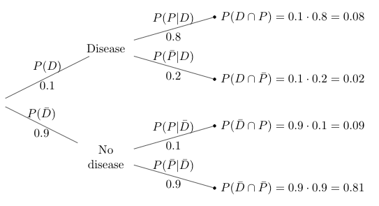
(The sum of all 4 scenarios must be equal to 1 since these 4 scenarios cover all possible cases.)
We are looking for the probability that an individual has the disease given that the result of the test is positive, \(P(D | P)\).
Following the formula of the conditional probability (Eq. 1) we have:
\[P(A | B) = \frac{P(A \cap B)}{P(B)}\]
In terms of our problem:
\[P(D | P) = \frac{P(D \cap P)}{P(P)}\] \[P(D | P) = \frac{0.08}{P(P)} \text{ (Eq. 4)}\]
From the tree diagram, we can see that a positive test result is possible under two scenarios:
- when a person has the disease, or
- when the person does not actually have the disease (because the test is not always correct).
In order to find the probability of a positive test result, \(P(P)\), we need to sum up those two scenarios:
\[\begin{align} P(P) &= P(D \cap P) + P(\bar{D} \cap P) \\ &= 0.08 + 0.09 \\ &= 0.17 \end{align}\]
Eq. 4 then becomes
\[P(D | P) = \frac{0.08}{0.17} = 0.4706\]
The probability of having the disease given that the result of the test is positive is only 47.06%. This means that in this specific case (with the same percentages), an individual with a positive test has less than 1 chance out of 2 of having the disease!
This relatively small percentage is due to the facts that the disease is quite rare (only 10% of the population is affected) and that the test is not always correct (sometimes it detects the disease although it is not present, and sometimes it does not detect it although it is present).
As a consequence, a higher percentage of healthy people have a positive result (9%) compared to the percentage of people who have a positive result and who actually have the disease (8%). This explains why several diagnostic tests are often performed before announcing the diagnosis, especially for rare diseases.
8. Accuracy measures
Based on the example of the disease and the diagnostic test presented above, we explain the most common accuracy measures:
- False negative (number and rate)
- False positive (number and rate)
- Sensitivity
- Specificity
- Positive predictive value
- Negative predictive value
Before diving into the details of these accuracy measures, here is an overview of the measures and the tree diagram with the labels added for each of the 4 scenarios:
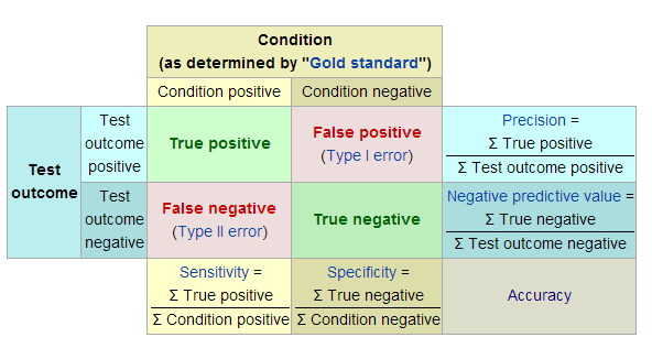
Adapted from Wikipedia
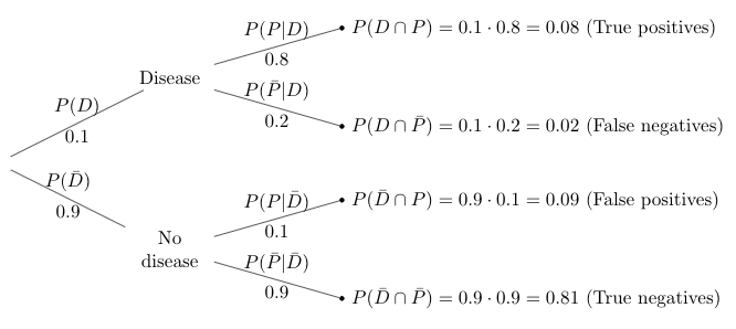
False negatives
The false negatives (FN) are the number of people incorrectly labeled as not having the disease or the condition, when in reality it is present. It is like telling a women who is 7 months pregnant that she is not pregnant.
From the tree diagram, we have:
\[FN = P(D \cap \bar{P}) = 0.02\]
Moreover, the false negative rate (FNR) is defined as
\[\begin{align} FNR &= \frac{FN}{FN + TP} \\ &= P(\bar{P} | D) \\ &= \frac{P(\bar{P} \cap D)}{P(D)} \\ &= \frac{0.02}{0.08 + 0.02} \\ &= 0.2 \end{align}\]
False positives
The false positives (FP) are the number of people incorrectly labeled as having the disease or the condition, when in reality it is not present. It is like telling a man he is pregnant.
From the tree diagram, we have:
\[FP = P(\bar{D} \cap P) = 0.09\]
Moreover, the false positive rate (FPR) is defined as
\[\begin{align} FPR &= \frac{FP}{FP + TN} \\ &= P(P | \bar{D}) \\ &= \frac{P(P \cap \bar{D})}{P(\bar{D})} \\ &= \frac{0.09}{0.09 + 0.81} \\ &= 0.1 \end{align}\]
Sensitivity
The sensitivity of a test, also referred as the recall, measures the ability of a test to detect the condition when the condition is present (the percentage of sick people who are correctly identified as having the disease):
\[ Sensitivity = \frac{TP}{TP + FN}\]
where TP is the true positives.
From the tree diagram, we have:
\[\begin{align} Sensitivity &= \frac{TP}{TP + FN} \\ &= P(P|D) \\ &= 0.8 \end{align}\]
Note also that \(1 - sensitivity = FNR\) (false negative rate).
Specificity
The specificity of a test measures the ability of a test to correctly exclude the condition when the condition is absent (the percentage of healthy people who are correctly identified as not having the disease):
\[Specificity = \frac{TN}{TN + FP}\]
where TN is the true negatives.
From the tree diagram, we have:
\[\begin{align} Specificity &= \frac{TN}{TN + FP} \\ &= P(\bar{P} | \bar{D}) \\ &= 0.9 \end{align}\]
Note also that \(1 - specificity = FPR\) (false positive rate).
Positive predictive value
The positive predictive value, also referred as the precision, is the proportion of positives that correspond to the presence of the condition, so the proportions of positive results that are true positive results:
\[PPV = \frac{TP}{TP+FP}\]
From the tree diagram, we have:
\[\begin{align} PPV &= \frac{TP}{TP+FP} \\ &= P(D | P) \\ &= \frac{P(D \cap P)}{P(P)} \\ &= \frac{0.08}{0.08+0.09} \\ &= 0.4706 \end{align}\]
Negative predictive value
The negative predictive value is the proportion of negatives that correspond to the absence of the condition, so the proportions of negative results that are true negative results:
\[NPV = \frac{TN}{TN + FN}\]
From the tree diagram, we have:
\[\begin{align} NPV &= \frac{TN}{TN + FN} \\ &= P(\bar{D} | \bar{P}) \\ &= \frac{P(\bar{D} \cap \bar{P})}{P(\bar{P})} \\ &= \frac{0.81}{0.81+0.02} \\ &= 0.9759 \end{align}\]
9. Counting techniques
In order to use the formula in section 2, one must know how to count the number of possible elements (both for favorable and possible cases).
There are 3 main counting techniques in probability:
- Multiplication
- Permutation
- Combination
See below how to count the number of possible elements in case of equiprobable results.
Multiplication
The multiplication rule is as follows:
\[\#(A \times B) = (\#A) \times (\#B)\]
where \(\#\) is the number of elements.
Example
In a restaurant, a customer has to choose a starter, a main course and a dessert. The restaurant offers 2 starters, 3 main courses and 2 desserts. How many different choices are possible?
There are \(2 \cdot 3 \cdot 2 = 12\) different possible choices.
Permutation
The number of permutations is as follows:
\[\begin{align} P^r_n &= n \times (n - 1) \times \cdots \times (n - r + 1) \\ &= \frac{n !}{(n - r)!} \end{align}\]
with \(r\) the length, \(n\) the number of elements and \(r \le n\). Note that \(0! = 1\) and \(k! = k \times (k - 1) \times (k - 2) \times \cdots \times 2 \times 1\) if \(k = 1, 2, \dots\)
The order is important in permutations!
Example
Count the permutations of length 2 of the set \(A = \{a, b, c, d\}\), without a letter being repeated. How many permutations do you find?
By hand
\[P^4_2 = \frac{4!}{(4-2)!} = \frac{4\cdot3\cdot2\cdot1}{2\cdot1} = 12\]
In R
library(gtools)

x <- c("a", "b", "c", "d")

# See all different permutations
perms <- permutations(
  n = 4, r = 2, v = x,
  repeats.allowed = FALSE
)
perms
## [,1] [,2]
## [1,] "a" "b"
## [2,] "a" "c"
## [3,] "a" "d"
## [4,] "b" "a"
## [5,] "b" "c"
## [6,] "b" "d"
## [7,] "c" "a"
## [8,] "c" "b"
## [9,] "c" "d"
## [10,] "d" "a"
## [11,] "d" "b"
## [12,] "d" "c"# Count the number of permutations
nrow(perms)## [1] 12Combination
The number of combinations is as follows:
\[\begin{align} C^r_n &= \frac{P^r_n}{r!} \\ &= \frac{n !}{r!(n - r)!} \\ &= {n \choose r} \\ &= \frac{n}{r} \times \frac{n - 1}{r - 1} \times \dots \times \frac{n - r + 1}{1} \end{align}\]
with \(r\) the length, \(n\) the number of elements and \(r \le n\).
The order is not important in combinations!
Example
In a family of 5 children, what is the probability that there are 3 girls and 2 boys? Assume that the probabilities of giving birth to a girl and a boy are equal.
By hand
- Count of 3 girls and 2 boys (favourable cases): \(C^3_5 = {5 \choose 3} = \frac{5!}{3!(5-3)!} = 10\)
- Count of possible cases: \(2^5 = 32\)
\(\Rightarrow P(3 \text{ girls and 2 boys}) = \frac{\text{# of favourable cases}}{\text{# of possible cases}}\) \[= \frac{10}{32} = 0.3125\]
In R
- Count of 3 girls and 2 boys:
choose(n = 5, k = 3)## [1] 10- Count of possible cases:
2^5## [1] 32Probability of 3 girls and 2 boys:
choose(n = 5, k = 3) / 2^5## [1] 0.3125Conclusion
Thanks for reading.
I hope this article helped you to understand the most important formulas and concepts from probability theory.
As always, if you have a question or a suggestion related to the topic covered in this article, please add it as a comment so other readers can benefit from the discussion.
Liked this post?
- Get updates every time a new article is published (no spam and unsubscribe anytime)
- Support the blog
- Share on:


